Statistical Inference: The Setup
- Data: x_1, \ldots, x_n observed
- Model: x_i \overset{iid}{\sim} f(x \mid \theta), with \theta unknown
- Three basic tasks:
- Point estimation: find a single value \hat\theta close to \theta
- Hypothesis testing: decide whether the data are compatible with H_0
- Bayesian inference: describe uncertainty about \theta via a distribution
Point Estimation
An estimator is a function of the data:
\hat\theta = \hat\theta(x_1, \ldots, x_n)
Familiar examples:
- Sample mean \hat\mu = \bar x = \frac{1}{n}\sum_{i=1}^n x_i
- Sample variance \hat\sigma^2 = S^2 = \frac{1}{n-1}\sum_{i=1}^n (x_i - \bar x)^2
- Least squares in regression \hat\beta = (X'X)^{-1} X' y
Evaluating an Estimator
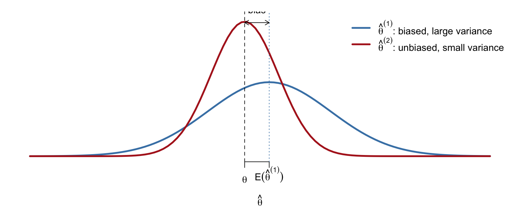
Since \hat\theta depends on random data, it has a sampling distribution.
![]()
- Bias E(\hat\theta) - \theta, variance V(\hat\theta), and \text{MSE}(\hat\theta) = E(\hat\theta - \theta)^2 = \text{Bias}^2 + V(\hat\theta)
- Comparing \hat\theta^{(1)} and \hat\theta^{(2)} requires knowing (or approximating) both sampling distributions
Maximum Likelihood Estimation
The log-likelihood of \theta:
\ell(\theta) = \log f(x_1, \ldots, x_n \mid \theta) = \log \prod_{i=1}^n f(x_i \mid \theta) = \sum_{i=1}^n \log f(x_i \mid \theta)
The MLE is the maximizer:
\hat\theta_{\text{MLE}} = \arg\max_\theta \ell(\theta)
- Closed form exists in simple models (normal mean, binomial proportion)
- In most models (GLMs, mixed models, survival models) there is no closed form
Hypothesis Testing
Test H_0: \mu = \mu_0 against H_1: \mu \neq \mu_0 using
T = \frac{\bar x - \mu_0}{S/\sqrt{n}}
- Need the null distribution of T (distribution of T when H_0 is true)
- For normal data, T \sim t_{n-1} exactly; for other data, the null distribution is known only approximately or not at all
p-value, Type I Error, and Power
![]()
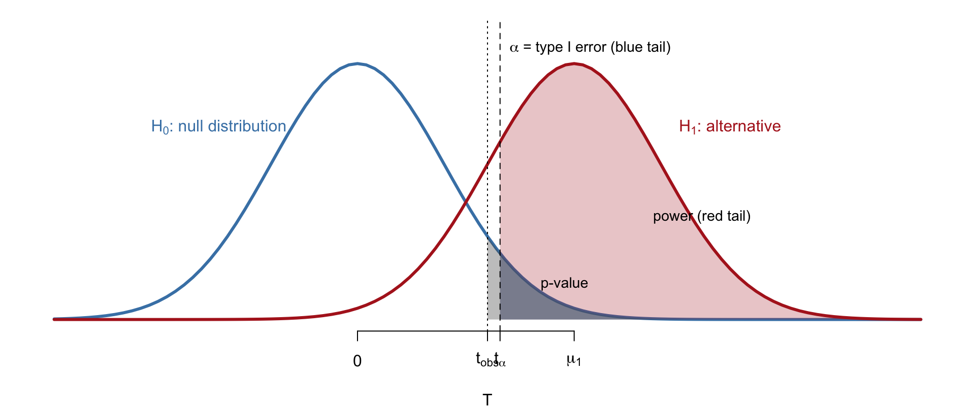
- p-value = P_{H_0}(T \ge t_{\text{obs}}): tail area of the null distribution beyond the observed statistic
- Type I error \alpha = P_{H_0}(T \ge t_\alpha): null tail area beyond the critical value
- Power = P_{H_1}(T \ge t_\alpha): alternative tail area beyond the critical value
All three are tail probabilities of a distribution that is often unknown in closed form.
Bayesian Inference
Combine a prior \pi(\theta) with the likelihood f(x \mid \theta):
p(\theta \mid x) = \frac{f(x \mid \theta)\,\pi(\theta)}{\int f(x \mid \theta)\,\pi(\theta)\, d\theta}
The denominator is an integral over \theta; for most models it has no closed form.
Prior, Likelihood, and Posterior
![]()
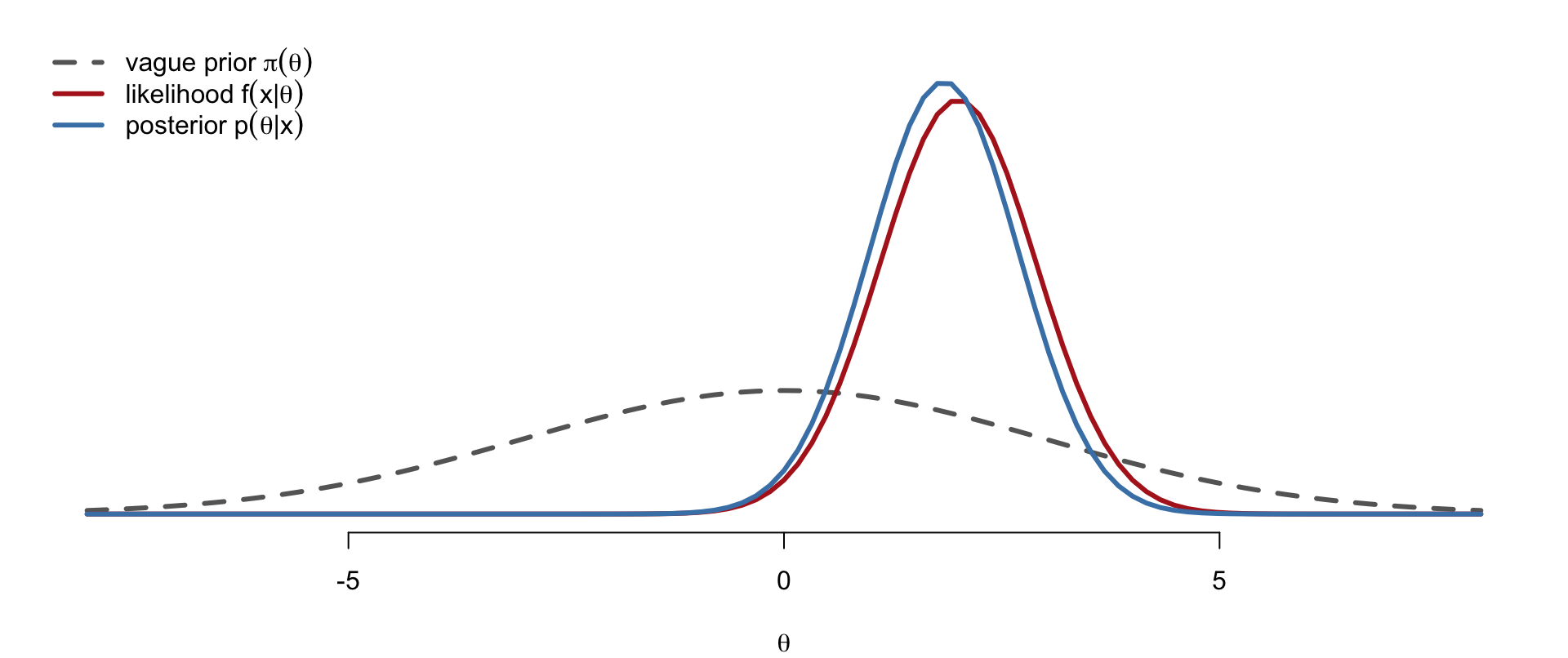
- A vague prior lets the likelihood dominate; the posterior is slightly narrower and pulled toward the prior mean
- Inference uses posterior summaries: E(\theta \mid x), V(\theta \mid x), credible intervals, P(H_0 \mid x)
- Each summary is again an integral over \theta
Summary of the Three Tasks
| Point estimation |
Sampling distribution of \hat\theta; maximizer of \ell(\theta) |
No closed form |
| Hypothesis testing |
Null distribution of T |
Unknown for general data |
| Bayesian inference |
\int f(x\mid\theta)\pi(\theta)\,d\theta; E(\theta \mid x) |
High-dimensional integral |
Each task reduces to a computational problem: calculating, simulating, optimizing, or integrating.
The Use of Computers in Statistics
1. Manipulating Numbers
Even simple calculations are not trivial on a computer:
- 1.1 + 2.1 + \cdots + 100.1
- S^2 = \sum_{i=1}^n (x_i - \bar x)^2 / (n-1)
- \prod_{i=1}^n f(x_i \mid \theta) for large n
Computers store numbers with finite precision, which leads to
- Overflow: result too large to represent
- Underflow: result too small, rounded to zero
- Rounding error: accumulated loss of digits
Example: Rounding Error
x <- c(1e10 + 1, 1e10 + 2, 1e10 + 3)
var(x)                                    # correct answer: 1
sum(x^2)/2 - 3 * mean(x)^2 / 2 # textbook formula
prod(dnorm(rnorm(1000))) # likelihood underflows to 0
sum(dnorm(rnorm(1000), log = TRUE)) # log-likelihood is fine
Lecture on computer arithmetic: how numbers are stored and how to avoid these errors.
2. Simulation with Random Numbers
Monte Carlo: replace a probability calculation with repeated random experiments.
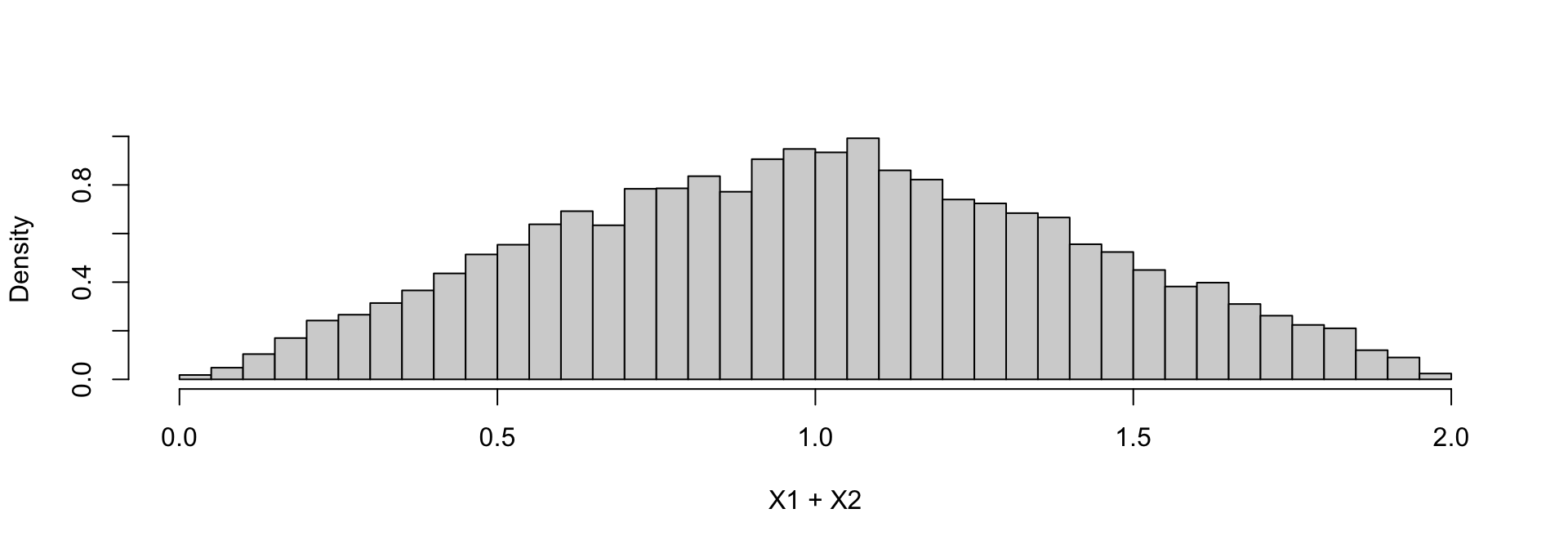
Generate X_1, X_2 \overset{iid}{\sim} \text{Unif}(0,1). What is the distribution of X_1 + X_2?
z <- runif(10000) + runif(10000)
hist(z, breaks = 40, freq = FALSE, main = "", xlab = "X1 + X2")
![]()
Monte Carlo for Sampling Distributions
Repeat many times: draw x_1, \ldots, x_n, compute the statistic.
\sum_i x_i, \qquad \sum_i (x_i - \bar x)^2, \qquad T = \frac{\bar x - \mu_0}{S/\sqrt n}
This gives empirical approximations to
- The sampling distribution of \hat\mu^{(1)} vs \hat\mu^{(2)} (bias, variance, MSE)
- The null distribution of T for non-normal data
- Coverage of confidence intervals
Lecture on random numbers and Monte Carlo: pseudo-random generation, transformations, LLN/CLT, evaluating estimators and tests.
3. Optimization
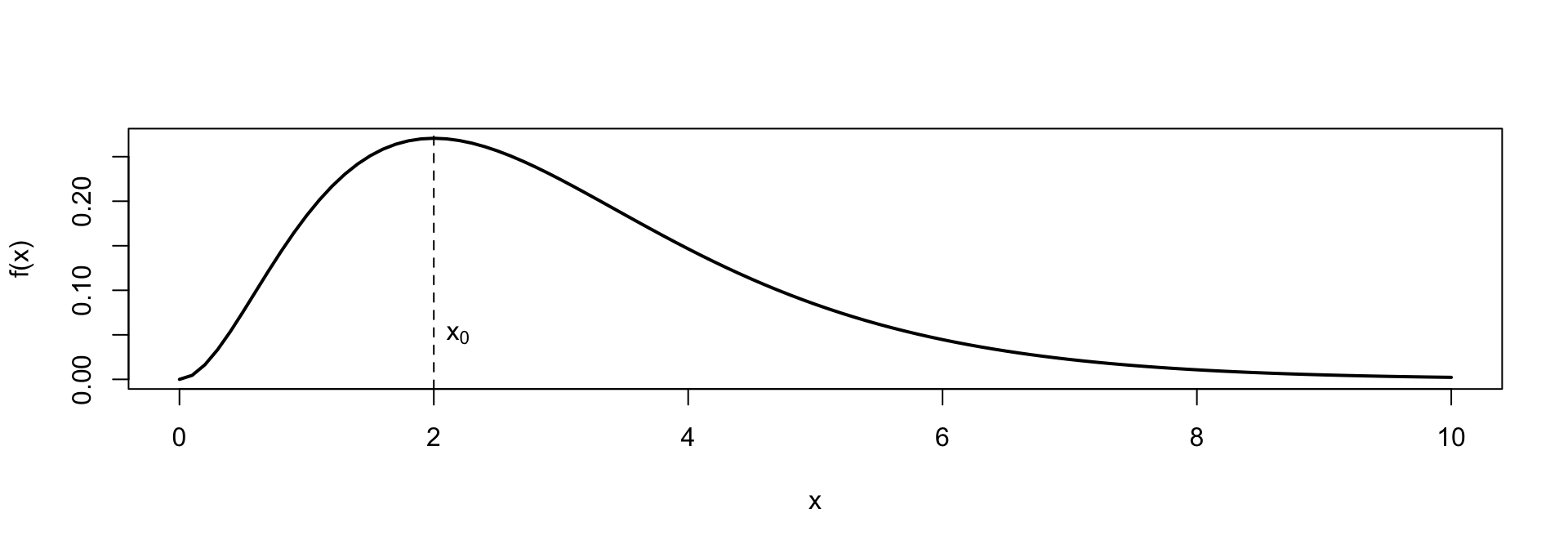
Find x_0 = \arg\max_x f(x).
![]()
For MLE, f = \ell(\theta); there is no closed form, so the maximum is found by iterative search.
Lecture on MLE and optimization: Newton–Raphson, Fisher scoring, Nelder–Mead, gradient methods, stochastic gradient descent.
4. Advanced Simulation and Integration
Quantities of interest are integrals:
E(X) = \int x f(x)\,dx, \qquad V(X), \qquad \int f(x\mid\theta)\pi(\theta)\,d\theta
Two approaches:
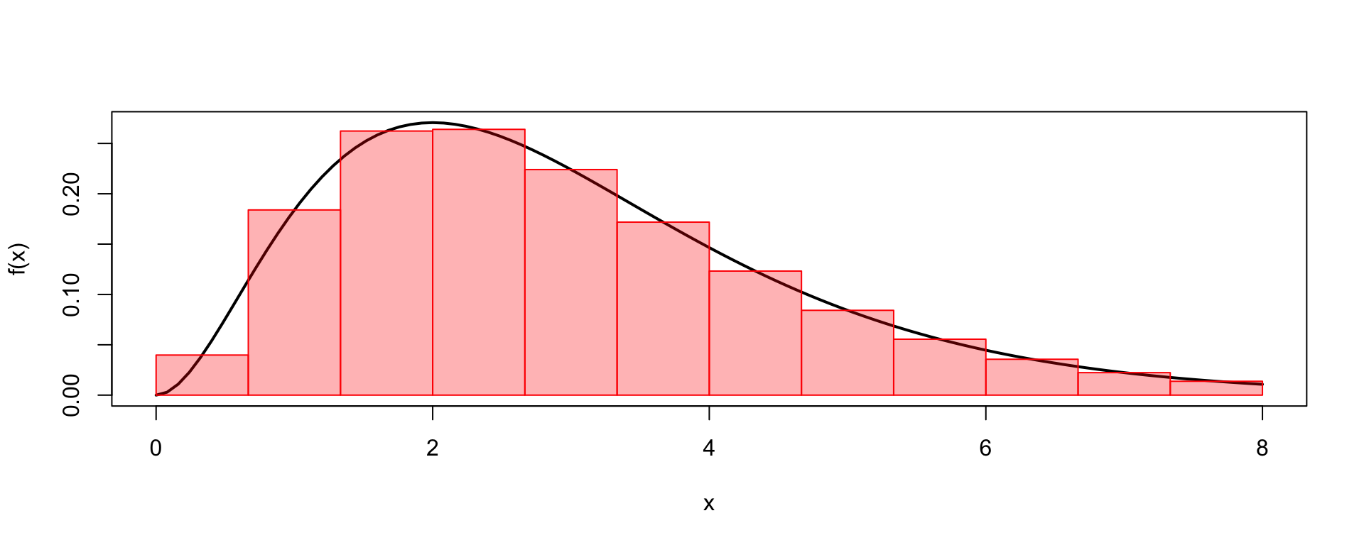
- Numerical quadrature: approximate the area under the curve by rectangles or trapezoids; works well in low dimension
- Monte Carlo integration: draw from f and average; the only practical route in high dimension
For the posterior p(\theta \mid x), direct sampling is impossible, so Markov chain Monte Carlo is used.
Numerical Quadrature
![]()
\int_a^b f(x)\,dx \approx \sum_{j=1}^k f(m_j)\,\Delta x
Course Roadmap
| Computer arithmetic |
Reliable calculation of likelihoods and variances |
| Random numbers and Monte Carlo |
Sampling distributions, evaluating estimators and tests |
| MLE and optimization |
Point estimation without closed forms |
| Numerical integration and MCMC |
Bayesian inference |
Throughout: R programming, vectorization, and efficient code.