Elements of Statistical Computation

Computer Arithmetic

2026-09-20

1 Representations of Numbers in Computer

Place Value

Every number is a string of digits in boxes; each box has a place value.

10³	10²	10¹	10⁰
1	3	4	8

1348 = 1\times10^3 + 3\times10^2 + 4\times10^1 + 8\times10^0

A computer uses base 2, so each box (a bit) holds 0 or 1:

2³	2²	2¹	2⁰
1	1	0	1

1101_2 = 1\times2^3 + 1\times2^2 + 0\times2^1 + 1\times2^0 = 13

Integers: Fixed Number of Boxes

An integer is stored in a fixed number of bits, e.g. 32 or 64. With p bits the largest unsigned value is \sum_{i=0}^{p-1} 2^i = 2^p - 1 .

A 4-bit example: the largest storable integer is 1111_2 = 15.

2⁴	2³	2²	2¹	2⁰
1	0	0	0	0

15 + 1 = 16 = 10000_2 needs a fifth box that does not exist → integer overflow

Integers: Fixed Number of Boxes (Continued)

R integers use 32 bits with one sign bit, so the largest is 2^{31}-1:

Code

.Machine$integer.max

[1] 2147483647

Code

.Machine$integer.max + 1L    # NA, with a warning

[1] NA

Unlike C, R does not wrap around silently — it returns NA. R also auto-promotes to double for most arithmetic, so overflow rarely bites unless both operands stay integer:

Code

50000L * 50000L   # integer * integer overflows

[1] NA

Code

50000 * 50000      # double: fine

[1] 2.5e+09

Floating Point Numbers: Scientific Notation in Boxes

A real number is stored as sign, mantissa (significant digits) and exponent: x = (-1)^{s} \times 1.d_1 d_2 \cdots d_p \times 2^{\,e}

sign	mantissa (fixed number of digits)					exponent
+	1	.	d₁	d₂ … d_p	×2^	±	e

Double precision (double in R) uses 64 bits:

part	bits	consequence
sign	1
mantissa	52	about 16 significant decimal digits
exponent	11	e \in [-1022,\ 1023], i.e. magnitudes from 10^{-308} to 10^{308}

A Toy Decimal Computer: Ruler and Zoom

A floating point number is a ruler and a zoom setting:

The mantissa is a ruler with a fixed number of equally spaced marks.
The exponent stretches the ruler by 10^{e} over [10^{e}, 10^{e+1}).
Stretching adds no marks — the marks spread apart as the zoom (exponent) grows.

Our toy computer stores six boxes: sign, a 2-digit mantissa d_1.d_2 (d_1\in\{1,\ldots,9\}, d_2\in\{0,\ldots,9\}), and a signed 1-digit exponent, e\in\{-9,\ldots,9\}:

sign	1		10⁻¹		±	exp
+	3	.	1	×10^	+	0

+3.1\times10^{+0} — the closest storable value to \pi

Zoom Levels: How Many Numbers Exist?

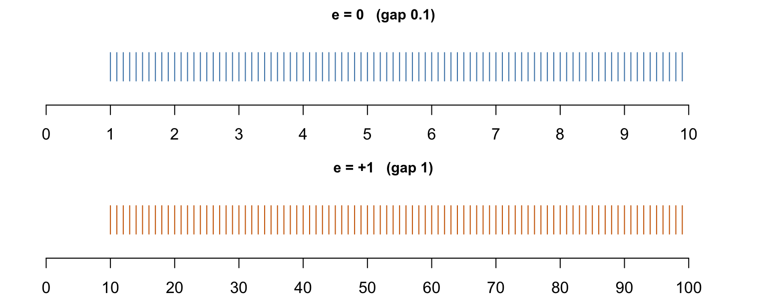
Each of the 19 zoom levels (e = -9,\ldots,9) is a ruler of 90 marks (1.0, 1.1, \ldots, 9.9). At the lowest zoom (e=-9) the leading digit may also be 0 — subnormal numbers — filling the gap between 0 and 1.0\times10^{-9}.

zoom e	interval	mantissa	magnitude	gap
-9 (subnormal)	(0, 10^{-9})	0.1,0.2,\ldots,0.9	\times10^{-9}	10^{-10}
-9	[10^{-9}, 10^{-8})	1.0,1.1,\ldots,9.9	\times10^{-9}	10^{-10}
\vdots	\vdots	\vdots	\vdots	\vdots
0	[1, 10)	1.0, 1.1, \ldots, 9.9	\times10^{0}	0.1
+1	[10, 100)	1.0,1.1,\ldots,9.9	\times10^{1}	1
\vdots	\vdots	\vdots	\vdots	\vdots
+9	[10^{9}, 10^{10})	1.0,1.1,\ldots,9.9	\times10^{9}	10^{8}

Visualizing the Zoom

Stretching by \times10 multiplies the gap by 10 — it does not add marks:

The absolute gap grows with magnitude; the relative gap stays roughly constant across zoom levels.

Rounding: Relative Error is Constant

A number that falls between two marks is stored as the nearer mark. These three numbers share the same mantissa digits and differ only in exponent (zoom):

x	stored	error
0.234	0.23	0.004 (1.7%)
2.34	2.3	0.04 (1.7%)
23.4	23	0.4 (1.7%)

Absolute error scales with the zoom; relative error does not — it is set by how many mantissa digits exist, not by magnitude.

Rounding in Addition: Machine Epsilon

To add, align by place value. Solid boxes are stored digits, dashed boxes are alignment zeros; digits beyond the mantissa (red) are rounded off.

	10⁰		10⁻¹	10⁻²
	1	.	0
+	0	.	1	0
	1	.	1	0

1.0+0.10=1.1 \ne 1.0

	10⁰		10⁻¹	10⁻²
	1	.	0
+	0	.	1	4
	1	.	1	4

1.0+0.14 \to 1.1

	10¹		10⁻¹	10⁻²
	1	.
+	0	.	4	0
	1	.	4	0

10+0.40 \to 10

Machine epsilon \epsilon = the gap next to 1 = the smallest increment the last mantissa box can register: here \epsilon = 0.1. Below it, digits are lost — partly (middle) or wholly (right, at a higher zoom).

Largest and Smallest Toy Numbers

	sign	mantissa	exponent	value
largest positive	+	9.9	+9	9.9\times10^{9}
smallest positive	+	0.1	-9	0.1\times10^{-9}
largest integer N with N+1 exact	+	9.9	+1	99

The first two set the range: anything above 9.9\times10^{9} overflows, anything below 1.0\times10^{-9} underflows.
The third is set by the precision: every integer up to 100 is representable, since 99+1 = 100 = 0.1\times10^{2}. But 100+1 = 101 needs three mantissa digits and rounds back to 100 — the same failure as 2^{53}+1 = 2^{53} in doubles, at 10^{2} instead of 2^{53}.

Overflow

Adding two large toy numbers can need an exponent the single digit cannot hold:

	10¹⁰	10⁹
		6
+		5
	1	1

6.0\times10^{9} + 5.0\times10^{9} = 1.1\times10^{+10}: exponent 10 needs two digits → overflow, stored as Inf

For doubles the largest value is \approx 1.8\times10^{308}:

Code

.Machine$double.xmax

[1] 1.797693e+308

Code

2^1024

[1] Inf

Underflow

A tiny result can fall outside the mantissa entirely:

	sign	1		10⁻¹	10⁻²		±	exp
	+	0	.	0	1	×10^	−	9

(0.1\times10^{-9})\times0.1 = 0.01\times10^{-9}: the digit 1 falls outside the mantissa → underflow, stored as 0

For doubles the smallest positive value is 2^{-1074}\approx 4.9\times10^{-324} (the smallest with full precision is 2^{-1022}\approx 2.2\times10^{-308}):

Code

.Machine$double.xmin

[1] 2.225074e-308

Code

2^-1075

[1] 0

2 Methods for Mitigating Rounding Error

Roundoff and Cancellation Errors

Each elementary operation (+,-,\times,/) carries a relative error of at most u = 2^{-53}. One is harmless; the concern is that many accumulate, or that an existing error is amplified.
Large + small: A + a returns exactly A once |a| < |A| \times 2^{-53}, since a falls below the gap between doubles near A. For larger |a|/|A| only the tail of a is lost — harmless once, but such losses build up over many additions.
Large − large: what matters is the answer d = A - B, not the size of A and B. If |d| < |A| \times 2^{-53}, the result is 0: A and B are already the same double. More generally, |d| \approx |A| \times 2^{-k} means the leading k bits cancel, leaving only 53-k meaningful bits — the subtraction adds no error, but the error already in A and B is now |A|/|d| times larger relative to the answer.

Extreme Examples

Machine epsilon. \epsilon = 2^{-52} is the gap between 1 and the next double; anything smaller than half that gap disappears when added to 1.

.Machine$double.eps      # 2^-52

[1] 2.220446e-16

1 + 1e-16 == 1           # 1e-16 < 2^-53, so the addition does nothing

[1] TRUE

Large + small at integer scale. Past 2^{53} the spacing between doubles is 2, so adding 1 to 2^{53} cannot be represented and is lost.

2^53 + 1 == 2^53

[1] TRUE

Large − large: 1-\Phi(10). The true answer is d \approx 7.62\times10^{-24}, far below |A|\times2^{-53} \approx 1.11\times10^{-16}. So pnorm(10) already rounds to exactly 1 before the subtraction, and the difference returns 0 — not one correct digit survives.

A <- 1; B <- pnorm(10);c(B = B, `A - B` = A - B, true_d = pnorm(10, lower.tail = FALSE))

           B        A - B       true_d 
1.000000e+00 0.000000e+00 7.619853e-24

pnorm(10, lower.tail = FALSE) evaluates the tail directly and returns all 16 digits without evaluating B

Example: Computing Sum by Avoiding Large + Small

Illustration

Compute 1.0 + 0.04 + 0.04 in our 2-digit-mantissa toy system (exact value 1.08).

Left to right, (1.0 + 0.04) + 0.04: each addition needs a third mantissa digit, so each rounds back to 1.0 (the same loss as 1.0+0.40\to1.0 shown earlier, just smaller). Both small terms are lost — result 1.0.

Small terms first, 1.0 + (0.04 + 0.04):

×10^

−

then 1.0 + 0.08 →

0.04+0.04=0.08 exactly, then 1.0+0.08\to1.1 — one roundoff, not an accumulating one.

Strategies for Computing Sum

Sort ascending. Add the smallest terms first, so that a partial sum never dwarfs the next term. Cheap, but requires the whole vector in advance, and still degrades for very long sums.
Pairwise summation. Sum halves recursively. Error grows like \log n rather than n, at no extra cost. This is what NumPy uses.
Kahan compensated summation. Carry the part rounded away at each step and add it back at the next: y \leftarrow x_i - c, \quad t \leftarrow s + y, \quad c \leftarrow (t - s) - y, \quad s \leftarrow t. Here c holds the discarded low-order bits: (t-s) is the part of y that was absorbed, so subtracting y leaves what was not. Roughly four times the work, but the error no longer grows with n.
Extended precision. Accumulate in a wider type. R’s sum() uses a long double accumulator — 64-bit mantissa on x86, though only 53-bit on Apple Silicon, where it therefore behaves like the naive loop.

Demonstration

kahan_sum <- function(x) {
  s <- 0; comp <- 0
  for (v in x) { y <- v - comp; t <- s + y; comp <- (t - s) - y; s <- t }
  s
}

x <- c(1, rep(1e-16, 1e4))           # exact sum: 1 + 1e-16*1e-4=1+1e-12

s <- 0; for (v in x) s <- s + v      # naive loop

c(naive   = s - 1,
  sorted  = sum(sort(x)) - 1,
  kahan   = kahan_sum(x) - 1,
  builtin = sum(x) - 1,
  exact   = 1e-12)

       naive       sorted        kahan      builtin        exact 
0.000000e+00 1.000089e-12 1.000089e-12 0.000000e+00 1.000000e-12

Each small term is below 2^{-53} relative to the running total, so the naive loop discards all 10^4 of them and returns exactly 1 — the entire tail is lost. Sorting, compensation, and the wider accumulator each recover the answer.

Example: Computing Variance by Avoiding Large − Large

Two algebraically identical formulas for the sum of squared deviations: \underbrace{\sum_{i=1}^{n}(x_i - \bar{x})^2}_{\text{two-pass}} \;=\; \underbrace{\sum_{i=1}^{n} x_i^2 - \frac{\left(\sum_i x_i\right)^2}{n}}_{\text{one-pass}}

The one-pass formula needs only \sum x_i and \sum x_i^2, computed in a single sweep of the data.
When the x_i are large but close together, \sum x_i^2 and (\sum x_i)^2/n are both huge and nearly equal: large − large.

Illustration

x = (1, 2, 3): deviations (-1, 0, 1), so \sum(x_i-\bar x)^2 = 2.

Shift by M = 10^{8}: x = (M+1, M+2, M+3). The deviations and the answer are unchanged, but the one-pass formula computes

\sum x_i^2 \approx 3\times10^{16}, \qquad \frac{(\sum x_i)^2}{n} \approx 3\times10^{16}, \qquad \text{difference} = 2.

With 16 significant digits, 3\times10^{16} is stored with a gap of about 4 between neighbours:

16 digits kept									lost
3	.	0	0	…	0	0	1	2	4	×10^16

The true answer, 2, lies entirely in the lost digit.

Code

x <- c(1, 2, 3) + 1e8
c(one_pass = sum(x^2) - sum(x)^2 / 3, two_pass = sum((x - mean(x))^2))

one_pass two_pass 
       0        2

Computing Variance: Gradual Failure

The one-pass error grows like \epsilon M^2 n, so it worsens continuously as the shift M grows — eventually giving a negative “variance”, which is impossible:

Code

var1 <- function(x) { n <- length(x); (sum(x^2) - sum(x)^2 / n) / (n - 1) }
M <- 10^(0:10)
t(sapply(M, function(m) { x <- c(1, 2, 3) + m; c(M = m, one_pass = var1(x)) }))

          M one_pass
 [1,] 1e+00        1
 [2,] 1e+01        1
 [3,] 1e+02        1
 [4,] 1e+03        1
 [5,] 1e+04        1
 [6,] 1e+05        1
 [7,] 1e+06        1
 [8,] 1e+07        1
 [9,] 1e+08        0
[10,] 1e+09        0
[11,] 1e+10   -32768

Solutions

Two-pass: compute \bar x first, then \sum (x_i - \bar x)^2. Deviations are small and of similar size, so no cancellation. (var() does this.)
Shifted one-pass: subtract any convenient constant c \approx \bar x (e.g. c = x_1) before applying the one-pass formula: \sum (x_i-\bar x)^2 = \sum (x_i - c)^2 - \frac{\left(\sum (x_i - c)\right)^2}{n}
Welford’s online algorithm updates \bar x_k and \sum_{i\le k}(x_i - \bar x_k)^2 one observation at a time; use it for streaming data.

Code

var_shifted <- function(x) { n <- length(x); d <- x - x[1]; (sum(d^2) - sum(d)^2 / n) / (n - 1) }
var_welford <- function(x) {
  m <- 0; S <- 0
  for (k in seq_along(x)) { m_old <- m; m <- m + (x[k] - m) / k; S <- S + (x[k] - m_old) * (x[k] - m) }
  S / (length(x) - 1)
}
x <- c(1, 2, 3) + 1e10
c(one_pass = var1(x), shifted = var_shifted(x), welford = var_welford(x))

one_pass  shifted  welford 
  -32768        1        1

Computing e^x: Fix by Reformulating

For x>0 all terms are positive, so no cancellation occurs. Therefore compute e^{-x} = \frac{1}{e^{x}}, \qquad x > 0 .

Code

taylor_exp <- function(x, K = 100) sum(x^(0:K) / factorial(0:K))
c(naive = taylor_exp(-50), reciprocal = 1 / taylor_exp(50), true = exp(-50))

       naive   reciprocal         true 
2.805096e+11 1.928750e-22 1.928750e-22

General principle: rearrange a formula so that quantities of similar magnitude and the same sign are combined; avoid computing a small result as the difference of two large numbers.

Example: Computing \log(1-e^{-u})

The problems

This kernel appears whenever a difference is taken on the log scale, since \log(e^{a} - e^{b}) = a + \log(1 - e^{-u}), \qquad u = a - b > 0.

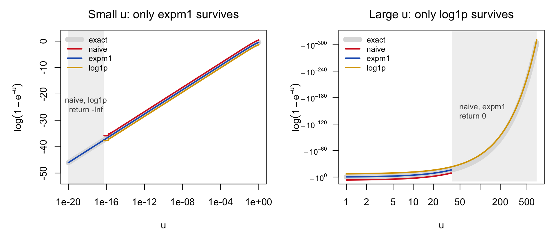
Evaluating it literally as log(1 - exp(-u)) fails at both ends of the range:

u small: e^{-u}\approx 1, so 1 - e^{-u} is large − large. The true value is \approx u, far below e^{-u}’s own rounding error, so the leading bits cancel and little survives — and for u < 2^{-53}, exp(-u) returns exactly 1 and the result is -\infty.
u large: e^{-u} is tiny, so 1 - e^{-u} is large + small. The small term is absorbed, 1-e^{-u} rounds to exactly 1, and log returns 0 instead of -e^{-u}.

The two incomplete remedies

R provides two functions built precisely for arguments near the landmark 1, each evaluating its series directly instead of forming the offending sum or difference:

expm1(x) computes e^{x}-1. For small x it returns \approx x with full precision, whereas exp(x) - 1 first rounds e^{x} to within 2^{-53} of 1 and then subtracts.
log1p(x) computes \log(1+x). For small x it returns \approx x with full precision, whereas log(1 + x) first rounds 1+x to exactly 1 and then takes the log.

Applied to compute \log(1-e^{-u}), each removes one of the two failures — and neither removes the other:

Code

f_naive <- function(u) log(1 - exp(-u))    # both failures
f_expm1 <- function(u) log(-expm1(-u))     # never forms the difference
f_log1p <- function(u) log1p(-exp(-u))     # never forms the sum

f_expm1 evaluates -\operatorname{expm1}(-u) = 1-e^{-u} without subtraction, fixing small u; its outer log then receives a value near u, far from 1, and is safe. f_log1p passes -e^{-u} straight to log1p, fixing large u; but for small u that argument has already rounded to -1.

Demonstration with Different u

Code

library(gt)
f_naive <- function(u) log(1 - exp(-u))    # both failures
f_expm1 <- function(u) log(-expm1(-u))     # never forms the difference
f_log1p <- function(u) log1p(-exp(-u))     # never forms the sum
log1mexp <- function(u) ifelse(u <= log(2), log(-expm1(-u)), log1p(-exp(-u))) # better solution 

u <- c(1e-100,1e-18, 1e-15,  1e-8, 1, 20, 50, 500)
g <- function(x) formatC(x, format = "g", digits = 8)

gt(data.frame(u = g(u), naive = g(f_naive(u)), expm1 = g(f_expm1(u)),
              log1p = g(f_log1p(u)), correct = g(log1mexp(u)))) |>
  tab_options(table.font.size = "30px")

u	naive	expm1	log1p	correct
1e-100	-Inf	-230.25851	-Inf	-230.25851
1e-18	-Inf	-41.446532	-Inf	-41.446532
1e-15	-34.539576	-34.538776	-34.539576	-34.538776
1e-08	-18.420681	-18.420681	-18.420681	-18.420681
1	-0.45867515	-0.45867515	-0.45867515	-0.45867515
20	-2.0611536e-09	-2.0611536e-09	-2.0611536e-09	-2.0611536e-09
50	0	0	-1.9287498e-22	-1.9287498e-22
500	0	0	-7.1245764e-218	-7.1245764e-218

Small u: naive tracks log1p — both lose digits, then collapse to -\infty. Only expm1 is right.
Large u: naive tracks expm1 — both collapse to 0. Only log1p is right.
Middle (10^{-8} \le u \le 20): all three agree; nothing is near a landmark.

Solution: `log1mexp`

Branch at u = \log 2, where e^{-u} = 1/2 — safely far from both traps:

Code

log1mexp <- function(u) ifelse(u <= log(2), log(-expm1(-u)), log1p(-exp(-u)))

The same function is shipped by several CRAN packages, all tracing to Mächler (2012).

Code

gt(data.frame(u      = g(u),
              naive  = g(f_naive(u)),
              mine   = g(log1mexp(u)),
              copula = g(copula::log1mexp(u)),
              VGAM   = g(VGAM::log1mexp(u)),
              DPQ    = g(DPQ::logspace.sub(0, -u)))) |>
  tab_options(table.font.size = "22px")

u	naive	mine	copula	VGAM	DPQ
1e-100	-Inf	-230.25851	-230.25851	-230.25851	-230.25851
1e-18	-Inf	-41.446532	-41.446532	-41.446532	-41.446532
1e-15	-34.539576	-34.538776	-34.538776	-34.538776	-34.538776
1e-08	-18.420681	-18.420681	-18.420681	-18.420681	-18.420681
1	-0.45867515	-0.45867515	-0.45867515	-0.45867515	-0.45867515
20	-2.0611536e-09	-2.0611536e-09	-2.0611536e-09	-2.0611536e-09	-2.0611536e-09
50	0	-1.9287498e-22	-1.9287498e-22	-1.9287498e-22	-1.9287498e-22
500	0	-7.1245764e-218	-7.1245764e-218	-7.1245764e-218	-7.1245764e-218

All four implementations agree to full precision across eighteen orders of magnitude, while the naive form is wrong at both ends. Prefer the package function in real code; write your own only to understand why it works.

The picture

Code

fin <- function(y) replace(y, !is.finite(y), NA)   # -Inf: the curve simply stops
## for the right panel: place y < 0 on a log axis without changing its sign,
## by plotting log10(-y) against a reversed axis labelled -10^k
negpow <- function(y) {
  out <- rep(NA_real_, length(y)); ok <- is.finite(y) & y < 0
  out[ok] <- log10(-y[ok]); out
}
cols <- c(naive = "#D62728", expm1 = "#1F5FBF", log1p = "#D9A400")
par(mfrow = c(1, 2), mar = c(4.2, 5.2, 2.6, 1), cex = 1.05)

## left: small u, value plotted directly; jitter in units of the response
u <- 10^seq(-20, 0, length.out = 400)
jit <- c(0.9, 0, -0.9)
plot(u, log1mexp(u), type = "n", log = "x", ylim = c(-52, 2),
     xlab = expression(u), ylab = expression(log(1 - e^-u)),
     main = expression("Small" ~ u * ": only expm1 survives"))
u_dead <- max(u[!is.finite(f_naive(u))])
rect(min(u), -60, u_dead, 10, col = adjustcolor("gray50", 0.12), border = NA)
text(sqrt(min(u) * u_dead), -24, "naive, log1p\nreturn -Inf", col = "gray30", cex = 0.8)
lines(u, log1mexp(u), lwd = 9, col = "gray87")
lines(u, fin(f_naive(u)) + jit[1], lwd = 2.5, col = cols["naive"])
lines(u, fin(f_expm1(u)) + jit[2], lwd = 2.5, col = cols["expm1"])
lines(u, fin(f_log1p(u)) + jit[3], lwd = 2.5, col = cols["log1p"])
legend("topleft", bty = "n", cex = 0.8, lwd = c(9, 2.5, 2.5, 2.5),
       col = c("gray87", cols), legend = c("exact", "naive", "expm1", "log1p"))

## right: large u, same quantity on a log-magnitude axis (note the reversed ylim);
## jitter is now in powers of ten, so it must be applied after negpow()
u <- 10^seq(0, log10(700), length.out = 400)
jit <- c(7, 0, -7)
k <- seq(0, -300, by = -60)
plot(u, negpow(log1mexp(u)), type = "n", log = "x", ylim = c(3, -320), yaxt = "n",
     xlab = expression(u), ylab = expression(log(1 - e^-u)),
     main = expression("Large" ~ u * ": only log1p survives"))
axis(2, at = k, labels = parse(text = paste0("-10^", k)), las = 1, cex.axis = 0.8)
u_dead <- min(u[f_naive(u) >= 0])
rect(u_dead, 10, max(u), -330, col = adjustcolor("gray50", 0.12), border = NA)
text(u_dead * 1.3, -150, "naive, expm1\nreturn 0", adj = c(0, 0.5), col = "gray30", cex = 0.8)
lines(u, negpow(log1mexp(u)), lwd = 9, col = "gray87")
lines(u, negpow(f_naive(u)) + jit[1], lwd = 2.5, col = cols["naive"])
lines(u, negpow(f_expm1(u)) + jit[2], lwd = 2.5, col = cols["expm1"])
lines(u, negpow(f_log1p(u)) + jit[3], lwd = 2.5, col = cols["log1p"])
legend("topleft", bty = "n", cex = 0.8, lwd = c(9, 2.5, 2.5, 2.5),
       col = c("gray87", cols), legend = c("exact", "naive", "expm1", "log1p"))

Figure 1: The three implementations against u on a log scale. Curves are offset vertically by a small constant so that they remain distinguishable where they agree; log1mexp is the grey reference.

3 Methods for Mitigating Overflow and Underflow Errors

Overflow and Underflow in Statistical Computing

Likelihoods are products of many probabilities; normalizing constants involve factorials or exponentials.

\prod_{i=1}^{2000} p(x_i) = \left(\tfrac12\right)^{2000} \approx 10^{-602} \quad\to\quad \text{underflow to } 0

1000! \approx 4\times10^{2567} \quad\to\quad \text{overflow to } \infty

\text{logistic: } \frac{e^{x}}{1+e^{x}} \text{ at } x = 1000 \quad\to\quad \frac{\infty}{\infty} = \texttt{NaN}

Two remedies: (1) change the algebraic expression; (2) work on the log scale.

Changing Algebraic Expression: The Sigmoid Function

Two equivalent forms: \sigma(x) = \frac{e^{x}}{1+e^{x}} = \frac{1}{1+e^{-x}}

x	e^{x}/(1+e^{x})	1/(1+e^{-x})
+1000	e^{x}=\infty, $/= $ `NaN` ✗	e^{-x}=0, 1/1 = 1 ✓
-1000	e^{x}=0, 0/1 = 0 ✓	e^{-x}=\infty, 1/\infty = 0 ✓

The second form never divides \infty by \infty.

Code

x <- 1000
c(naive = exp(x) / (1 + exp(x)), stable = 1 / (1 + exp(-x)))

 naive stable 
   NaN      1

Representing Numbers in Logarithmic Form

Represent a positive number x by \ell_x = \log x: x = e^{2000} \iff \ell_x = 2000, \qquad x = e^{-2000} \iff \ell_x = -2000 .

Numbers that overflow or underflow in ordinary form are ordinary numbers on the log scale.

We then need each operation f translated to the log scale: x_1,\dots,x_n \xrightarrow{\;f\;} y \qquad\Longleftrightarrow\qquad \ell_1,\dots,\ell_n \xrightarrow{\;\tilde f\;} \ell_y = \log f(e^{\ell_1},\dots,e^{\ell_n})

Products and Quotients on the Log Scale

\log(x_1 x_2) = \ell_1 + \ell_2, \qquad \log\left(\prod_{i=1}^{n} x_i\right) = \sum_{i=1}^{n} \ell_i, \qquad \log\frac{x_1}{x_2} = \ell_1 - \ell_2

Log-likelihood: \log \prod_i p(x_i) = \sum_i \log p(x_i) — always compute the log-likelihood, never the likelihood.

Example: x_1 = 2^{2000}, x_2 = 2^{2001} both overflow, but \log\frac{x_1}{x_2} = 2000\log 2 - 2001\log 2 = -\log 2 .

Code

c(direct = 2^2000 / 2^2001, log_scale = exp(2000 * log(2) - 2001 * log(2)))

   direct log_scale 
      NaN       0.5

The Log-Sum-Exp Trick

Sums are the hard case: \log(x_1 + x_2) \neq \ell_1 + \ell_2. We need \log\left(\sum_{i=1}^{n} x_i\right) = \log\left(\sum_{i=1}^{n} e^{\ell_i}\right), but the e^{\ell_i} may overflow or underflow. Let m = \max_i \ell_i and factor it out: \log\left(\sum_{i=1}^{n} e^{\ell_i}\right) = \log\left(e^{m}\sum_{i=1}^{n} e^{\ell_i - m}\right) = m + \log\left(\sum_{i=1}^{n} e^{\ell_i - m}\right) One dominant term: the sum becomes 1 + (\text{tiny}), and use log1p: \log(e^{a} + e^{b}) = m + \operatorname{log1p}\!\left(e^{-|a-b|}\right), \qquad m = \max(a,b).

Code

c(naive = log(exp(0) + exp(-50)),
  log1p = log1p(exp(-50)),
  exact = 1.93e-22)

      naive       log1p       exact 
0.00000e+00 1.92875e-22 1.93000e-22

Log-Sum-Exp: Illustration

x_i = e^{2000}, e^{2001}, e^{2002} — each overflows to Inf, so \sum x_i computed directly is Inf.

	i=1	i=2	i=3
\ell_i	2000	2001	2002
\ell_i - m (m = 2002)	-2	-1	0
e^{\ell_i - m}	0.135	0.368	1

\log\sum_i x_i = 2002 + \log(0.135 + 0.368 + 1) = 2002.408

Code

log_sum_exp <- function(l) { m <- max(l); m + log(sum(exp(l - m))) }
c(direct = log(sum(exp(c(2000, 2001, 2002)))), lse = log_sum_exp(c(2000, 2001, 2002)))

  direct      lse 
     Inf 2002.408

Applications: marginal likelihoods \log\sum_k \pi_k p_k(x) in mixtures, posterior normalizing constants, softmax.

Difference on the Log Scale

For x > y > 0 with \ell_x = \log x, \ell_y = \log y: \log(x - y) = \log\left(e^{\ell_x}\left(1 - e^{\ell_y - \ell_x}\right)\right) = \ell_x + \log\left(1 - e^{\ell_y - \ell_x}\right)

Since \ell_y - \ell_x < 0, e^{\ell_y-\ell_x}\in(0,1): no overflow.
When x \approx y, use log1p(-exp(ly - lx)) to avoid the cancellation in 1 - e^{\ell_y-\ell_x}.

Code

log_diff_exp <- function(lx, ly) lx + log1p(-exp(ly - lx))   # requires lx >= ly
log_diff_exp(2020, 2000)

[1] 2020

Code

log_diff_exp <- function(lx, ly) lx + log1p(-exp(ly - lx))   # requires lx >= ly
log_diff_exp(2020, 2019)

[1] 2019.541

Software implementation: logSumExp in matrixStats

The log-sum-exp trick is already implemented in matrixStats (used by hundreds of CRAN/Bioconductor packages):

Code

c(mine = log_sum_exp(c(2000, 2001, 2002)),
  matrixStats = matrixStats::logSumExp(c(2000, 2001, 2002)))

       mine matrixStats 
   2002.408    2002.408

For two terms, DPQ gives the log-scale counterpart of +, taken from R’s own pgamma() C code:

Code

c(naive = log(exp(2000) + exp(1999)),          # Inf + Inf
  DPQ   = DPQ::logspace.add(2000, 1999))

   naive      DPQ 
     Inf 2000.313

Use logspace.add() for a pair, logSumExp() for a vector.

Software implementation: log-difference in DPQ

logspace.sub(lx, ly) computes \log(e^{lx} - e^{ly}), the log-scale counterpart of subtraction, and logspace.add() does the same for the sum. Four extreme cases of u = lx - ly:

Code

library(DPQ)
lx <- c( 2000, 1e-20, -1000,   0)
ly <- c( 1999,     0, -1001, -500)

cbind(lx, ly, u = lx - ly,
      naive = log(exp(lx) - exp(ly)),
      DPQ   = logspace.sub(lx, ly))

         lx    ly     u naive            DPQ
[1,]  2e+03  1999 1e+00   NaN   1.999541e+03
[2,]  1e-20     0 1e-20  -Inf  -4.605170e+01
[3,] -1e+03 -1001 1e+00  -Inf  -1.000459e+03
[4,]  0e+00  -500 5e+02     0 -7.124576e-218

computing	u = a-b	e^{a} - e^{b} in doubles	naive `log()`	`logspace.sub`
\log(e^{2000} - e^{1999})	1	`Inf - Inf` → `NaN`	`NaN`	1999.54
\log(e^{10^{-20}} - e^{0})	10^{-20}	`1 - 1` → `0`	-\infty	-46.05
\log(e^{-1000} - e^{-1001})	1	`0 - 0` → `0`	-\infty	-1000.46
\log(e^{0} - e^{-500})	500	`1 - 1.93e-22` → `1`	0	-1.93\times10^{-22}

The third column is the whole story: the subtraction has been destroyed before log is ever called — by overflow, cancellation, underflow, and absorption respectively. The naive expression returns a wrong answer — silently, in three of four cases — across the whole range: for operands too large, too small, too close, and too far apart.

4 A Final Example

A List of Stable R Functions

Software provides functions written specifically to avoid rounding error, underflow, and overflow.

instead of	use	reason	solution
`log(1 + x)`	`log1p(x)`	for tiny x, `1 + x` rounds to 1	Taylor series x - \frac{x^2}{2} + \cdots
`exp(x) - 1`	`expm1(x)`	for tiny x, `exp(x)` rounds to 1	Taylor series x + \frac{x^2}{2} + \cdots
`log(factorial(n))`	`lfactorial(n)`, `lgamma(n + 1)`	`factorial(n)` overflows	Stirling series
`log(choose(n, k))`	`lchoose(n, k)`	overflow	sum of `lgamma` terms
`log(dnorm(x))`	`dnorm(x, log = TRUE)`	`dnorm(x)` underflows	closed-form log density
`log(pnorm(x))`	`pnorm(x, log.p = TRUE)`	underflow	asymptotic expansion
`log(1 - pnorm(x))`	`pnorm(x, lower.tail = FALSE, log.p = TRUE)`	cancellation and underflow	upper tail computed directly

Example: Computing \log(1-\Phi(10))

c(naive    = log(1 - pnorm(10)),     # pnorm(10) rounds to 1, so log(0) = -Inf
  log1p    = log1p(-pnorm(10)),      # log1p cannot recover digits already lost
  log1mexp = log1mexp(-pnorm(10, log.p = TRUE)),        # complement in log space
  stable   = pnorm(10, lower.tail = FALSE, log.p = TRUE))  # direct upper tail

    naive     log1p  log1mexp    stable 
     -Inf      -Inf -53.23129 -53.23129

The target is \log\{1 - \Phi(10)\} \approx -53.23, where 1 - \Phi(10) \approx 7.6 \times 10^{-24} is far below machine epsilon (\approx 2.2 \times 10^{-16}).

naive and log1p. pnorm(10) rounds to exactly 1, so the small difference is lost before any logarithm is taken. log1p preserves accuracy only for arguments that are themselves accurate.
log1mexp. Work from \ell = \log\Phi(10) \approx -7.6\times10^{-24}, which R returns accurately. \log\{1-\Phi(10)\} = \log(1 - e^{\ell}) = \log(1 - e^{-u}) = \texttt{log1mexp}(u), and since u is tiny the expm1 branch applies.
stable. With lower.tail = FALSE, R computes 1 - \Phi(10) directly, never forming \Phi(10), and log.p = TRUE returns its logarithm without underflow. A computing method is to apply log-sum-exp to the \log (\texttt{dnorm}(x)).

Example: Computing \log(1-\Phi(-10))

c(naive    = log(1 - pnorm(-10)),    # 1 - 7.6e-24 rounds to 1, so log gives 0
  log1p    = log1p(-pnorm(-10)),     # pnorm(-10) is accurate, so log1p is exact
  log1mexp = log1mexp(-pnorm(-10, log.p = TRUE)),
  stable   = pnorm(-10, lower.tail = FALSE, log.p = TRUE))

        naive         log1p      log1mexp        stable 
 0.000000e+00 -7.619853e-24 -7.619853e-24 -7.619853e-24

Here \Phi(-10) \approx 7.6 \times 10^{-24} and the target is \log\{1 - \Phi(-10)\} \approx -7.6 \times 10^{-24}, a tiny negative number rather than a large one.

naive. The subtraction 1 - 7.6 \times 10^{-24} rounds to exactly 1, so every significant digit is destroyed and the answer is reported as 0.
log1p. The argument pnorm(-10) is itself accurate, since a number near zero is represented with full relative precision. log1p then evaluates \log(1 + x) by its Taylor series without ever forming 1 + x, recovering all digits.
log1mexp. Now \ell = \log\Phi(-10) \approx -53.23, so u = 53.23 and the log1p branch applies. The same call is correct in both examples — only the branch differs.
stable. Also correct, and preferable in general.

Remarks

The contrast between the two examples is the location of the loss. At x=10 the damage occurs inside pnorm(10) before log1p is reached, so no reformulation of the outer expression helps. At x=-10 only the outer subtraction is unstable, which is what log1p is for.

The general lesson: stay on the log scale throughout. Ask R for \log\Phi rather than \Phi, and take the complement with log1mexp, which selects the right branch automatically. The tail direction then no longer needs to be diagnosed by hand.

Summary

Integers occupy a fixed number of bits; exceeding 2^{31}-1 gives NA with a warning in R (not silent wraparound as in C).
Doubles store sign + 52-bit stored mantissa (53 effective, ~16 decimal digits) + 11-bit exponent, covering roughly 10^{-308} to 10^{308}. The relative spacing varies between 2^{-53} and 2^{-52} within each binade, and integers above 2^{53} are not all representable.
Overflow → Inf; underflow → 0 (silent, and thus more dangerous).
Roundoff is amplified by large + small (fix: add small terms first, pairwise/Kahan summation) and large − large (fix: reformulate so the answer is never obtained as a difference of near-equal numbers — \sqrt{x+1}-\sqrt{x} = 1/(\sqrt{x+1}+\sqrt{x}), two-pass variance).
Overflow/underflow are avoided by working on the log scale, using purpose-built functions (log1p, expm1, lgamma, dnorm(log=TRUE))(log-sum-exp).

Elements of Statistical Computation

1 Representations of Numbers in Computer

Place Value

Integers: Fixed Number of Boxes

Integers: Fixed Number of Boxes (Continued)

Floating Point Numbers: Scientific Notation in Boxes

A Toy Decimal Computer: Ruler and Zoom

Zoom Levels: How Many Numbers Exist?

Visualizing the Zoom

Rounding: Relative Error is Constant

Rounding in Addition: Machine Epsilon

Largest and Smallest Toy Numbers

Overflow

Underflow

2 Methods for Mitigating Rounding Error

Roundoff and Cancellation Errors

Extreme Examples

Example: Computing Sum by Avoiding Large + Small

Illustration

Strategies for Computing Sum

Demonstration

Example: Computing Variance by Avoiding Large − Large

Illustration

Computing Variance: Gradual Failure

Solutions

Computing e^x: Fix by Reformulating

Example: Computing \log(1-e^{-u})

The problems

The two incomplete remedies

Demonstration with Different u

Solution: log1mexp

The picture

3 Methods for Mitigating Overflow and Underflow Errors

Overflow and Underflow in Statistical Computing

Changing Algebraic Expression: The Sigmoid Function

Representing Numbers in Logarithmic Form

Products and Quotients on the Log Scale

The Log-Sum-Exp Trick

Log-Sum-Exp: Illustration

Difference on the Log Scale

Software implementation: logSumExp in matrixStats

Software implementation: log-difference in DPQ

4 A Final Example

A List of Stable R Functions

Example: Computing \log(1-\Phi(10))

Example: Computing \log(1-\Phi(-10))

Remarks

Summary

Solution: `log1mexp`