A computer is deterministic, so it cannot produce truly random numbers. It produces pseudo random numbers: a deterministic sequence that behaves like iid \mathrm{Unif}(0,1) draws.
A classic generator, the linear congruential generator (LCG):
x_{i+1} = (a\,x_i + c) \bmod m, \qquad u_{i+1} = x_{i+1}/m
The starting value x_0 is the seed. The same seed gives the same sequence, which makes simulations reproducible.
The sequence eventually repeats; a good generator has a very long period and passes statistical tests of uniformity and independence.
R’s default is the Mersenne Twister (period 2^{19937}-1). All other distributions in R are built from \mathrm{Unif}(0,1) draws.
Code
lcg <-function(n, seed, a =69069, c =1, m =2^32) { x <-numeric(n); x[1] <- seedfor (i in2:n) x[i] <- (a * x[i -1] + c) %% m x / m}round(lcg(5, seed =812), 4)
[1] 0.0000 0.0131 0.9086 0.8102 0.2842
Pseudo Random Numbers: A Trace
Code
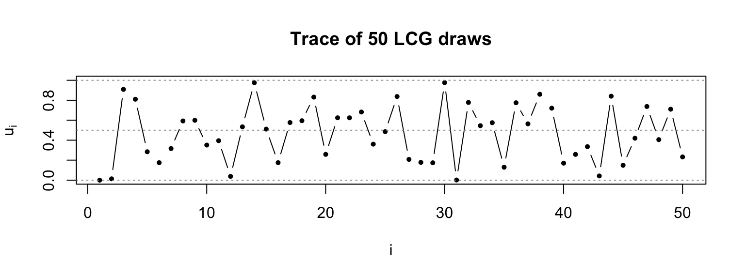
u <-lcg(50, seed =812)plot(u, type ="b", pch =16, cex =0.7, ylim =c(0, 1),xlab ="i", ylab =expression(u[i]),main ="Trace of 50 LCG draws")abline(h =c(0, 0.5, 1), lty =3, col ="grey60")
The trace shows no visible trend, drift, or periodicity, and the points fill (0,1) without clustering. This is what “behaves like iid uniform” means in practice, though a convincing assessment requires formal tests of uniformity and serial correlation rather than a single plot of 50 values.
Seeds and Reproducibility
set.seed(1); runif(3)
[1] 0.2655087 0.3721239 0.5728534
set.seed(1); runif(3) # identical
[1] 0.2655087 0.3721239 0.5728534
runif(3) # continues the sequence
[1] 0.9082078 0.2016819 0.8983897
Always set.seed() at the top of a simulation study so results can be reproduced and debugged.
Example: Generating \mathrm{Unif}(a,b)
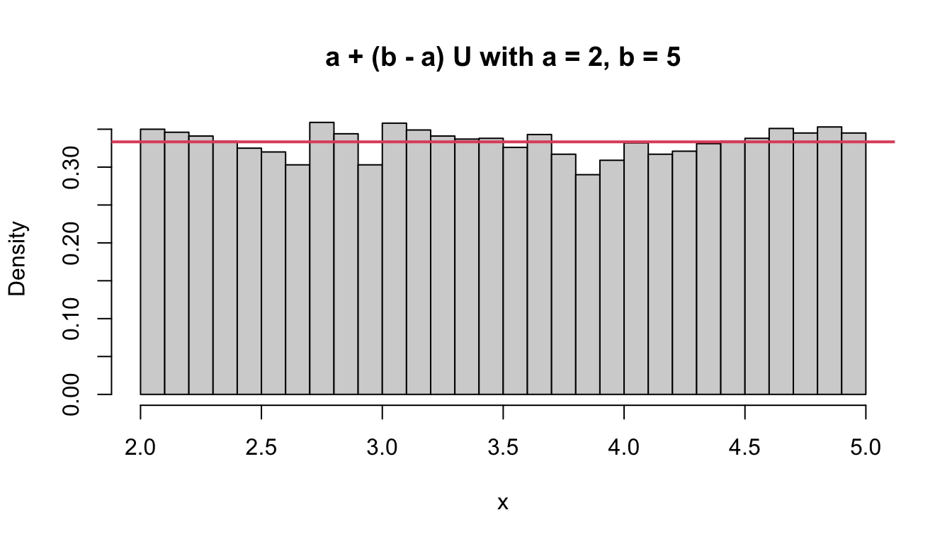
If U \sim \mathrm{Unif}(0,1) then X = a + (b-a)\,U \sim \mathrm{Unif}(a,b):
P(X \le x) = P\!\left(U \le \frac{x-a}{b-a}\right) = \frac{x-a}{b-a}, \qquad a \le x \le b .
u <-runif(10000); x <-2+3* u # Unif(2, 5)hist(x, breaks =30, freq =FALSE, main ="a + (b - a) U with a = 2, b = 5")abline(h =1/3, col =2, lwd =2)
Inverting the CDF (Continuous Case)
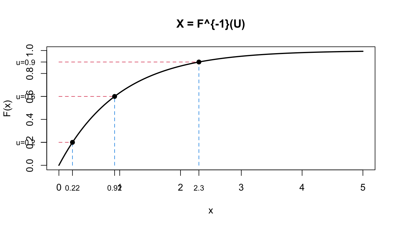
Let F_X be a continuous CDF with inverse (quantile function) F_X^{-1}.
Theorem. If U \sim \mathrm{Unif}(0,1), then X = F_X^{-1}(U) has CDF F_X.
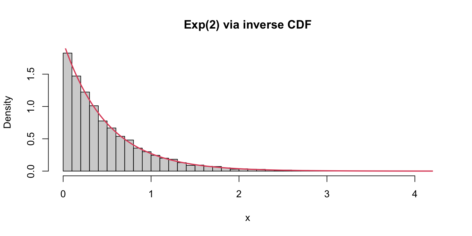
hist(x, breaks =40, freq =FALSE, main ="Exp(2) via inverse CDF")curve(dexp(x, lambda), add =TRUE, col =2, lwd =2)
A Transformation for Generating Normal Samples
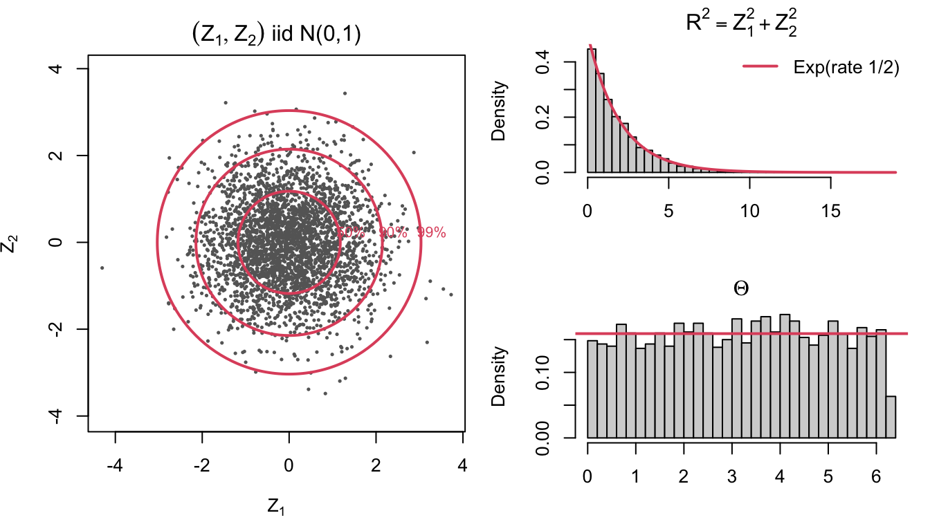
\Phi^{-1} has no closed form, so the inverse-CDF method is not directly usable. Instead, look at a pair (Z_1, Z_2) \overset{iid}{\sim} N(0,1) in polar coordinates:
Z_1 = R\cos\Theta, \qquad Z_2 = R\sin\Theta, \qquad R^2 = Z_1^2 + Z_2^2, \quad \Theta = \operatorname{atan2}(Z_2, Z_1).
The joint density \frac{1}{2\pi}e^{-(z_1^2+z_2^2)/2} depends on (z_1, z_2) only through r^2 = z_1^2 + z_2^2, so it is rotationally symmetric about the origin. Consequently:
The angle \Theta \sim \mathrm{Unif}(0, 2\pi), independent of R.
The squared radius R^2 = Z_1^2 + Z_2^2 \sim \chi^2_2, and \chi^2_2is the exponential distribution with rate 1/2:
f_{\chi^2_2}(w) = \frac{1}{2}e^{-w/2}, \quad w > 0 \qquad\Longrightarrow\qquad R^2 \sim \mathrm{Exp}(\text{rate} = 1/2).
Both R^2 and \Thetacan be generated by inverting a CDF.
Illustration: Two Standard Normals in Polar Coordinates
The point cloud is rotationally symmetric: the red circles enclose 50%, 90%, 99% of the points (R^2 \le \chi^2_2 quantiles); the angle is uniform; R^2 follows \mathrm{Exp}(1/2).
The Box–Muller Transformation
Reverse the picture: generateR^2 and \Theta, then rotate back to (Z_1, Z_2).
R^2 \sim \mathrm{Exp}(1/2) by inverse CDF: F(w) = 1 - e^{-w/2}, so R^2 = -2\log U_1, i.e. R = \sqrt{-2\log U_1}.
Theorem (Box–Muller). If U_1, U_2 \overset{iid}{\sim} \mathrm{Unif}(0,1), then.
Z_1 = \sqrt{-2\log U_1}\,\cos(2\pi U_2), \qquad Z_2 = \sqrt{-2\log U_1}\,\sin(2\pi U_2),
are independent N(0,1). Two uniforms produce two normals. Then \mu + \sigma Z \sim N(\mu, \sigma^2).
Box–Muller in R
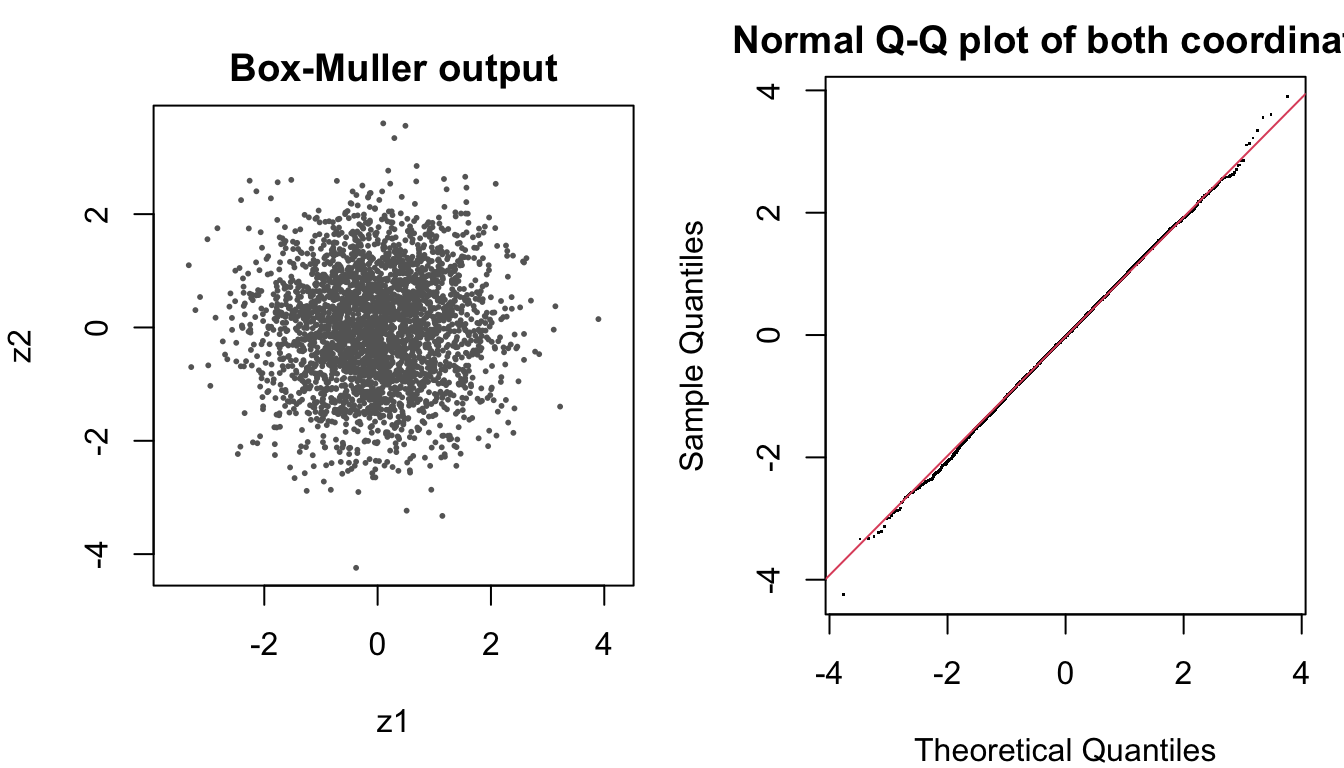
box_muller <-function(n) { u1 <-runif(n); u2 <-runif(n) r <-sqrt(-2*log(u1)) # R^2 ~ Exp(1/2), i.e. chi-square(2) th <-2* pi * u2 # Theta ~ Unif(0, 2 pi)cbind(z1 = r *cos(th), z2 = r *sin(th))}z <-box_muller(3000)par(mfrow =c(1, 2), mar =c(4, 4, 2, 1))par(pty ="s"); plot(z, pch =20, cex =0.4, col ="grey40", asp =1, main ="Box-Muller output")par(pty ="m"); qqnorm(c(z), pch =".", main ="Normal Q-Q plot of both coordinates"); qqline(c(z), col =2)
c(mean =mean(z), sd =sd(z), corr =cor(z)[1, 2])
       mean          sd        corr
-0.02673691  0.98937455  0.02537785
2 Monte Carlo Integration
Law of Large Numbers and Central Limit Theorem
Monte Carlo estimates an expectation \mu = E(g(X)) by an average of simulated values,
\hat\mu_n = \frac{1}{n}\sum_{i=1}^n g(X_i), \qquad X_i \overset{iid}{\sim} f .
Theorem (Strong Law of Large Numbers). If X_1, X_2, \ldots are iid with finite mean \mu, then.
P\left(\frac{X_1 + \cdots + X_n}{n} \to \mu\right) = 1 .
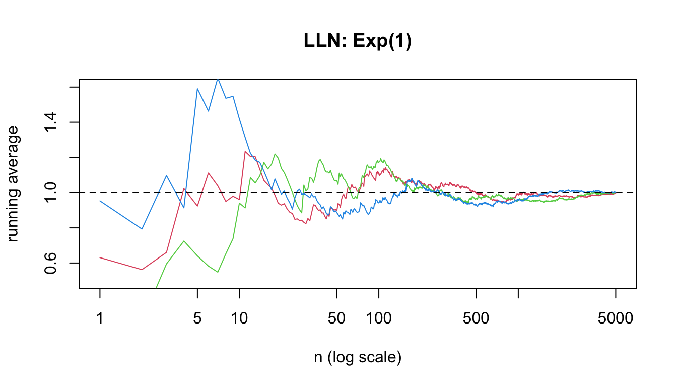
The LLN guarantees that the average converges to the truth. It does not say how fast.
Theorem (Central Limit Theorem). If in addition the variance \sigma^2 is finite, then
\frac{\overline X - \mu}{\sigma/\sqrt n} \;\xrightarrow{d}\; N(0,1).
The CLT gives the error bound: the Monte Carlo error is of order \sigma/\sqrt n.
Monte Carlo Error Bound from the CLT
From (5.2), with confidence level 95%,
P\!\left(\lvert\overline X - \mu
\rvert \le 1.96\,\frac{\sigma}{\sqrt n}\right) \approx 0.95,
so a 95% interval for \mu is
\overline X \pm 1.96\,\frac{\sigma}{\sqrt n}, \qquad \sigma \text{ replaced by the sample SD } s .
Halving the error requires four times as many samples; each extra decimal digit of accuracy costs a 100-fold increase in n.
The rate n^{-1/2} does not depend on the dimension of X, which is why Monte Carlo beats numerical quadrature in high dimensions.
Demonstration of the LLN
Running averages of X_i \sim \mathrm{Exp}(1) (\mu = 1) for three independent sequences:
n <-5000plot(NULL, xlim =c(1, n), ylim =c(0.5, 1.6), log ="x",xlab ="n (log scale)", ylab ="running average", main ="LLN: Exp(1)")for (k in1:3) lines(cumsum(rexp(n)) / (1:n), col = k +1)abline(h =1, lty =2)
Demonstration of the CLT
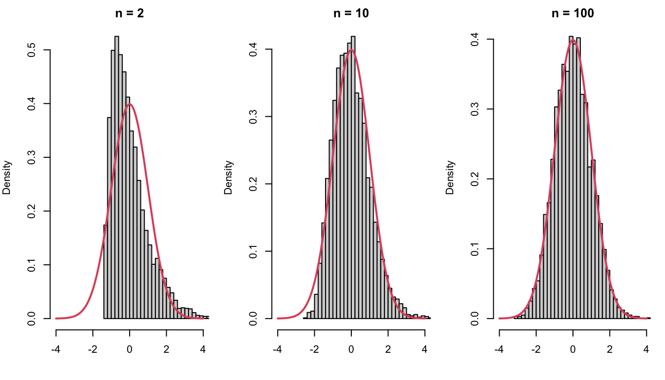
For each of N = 5000 repetitions, draw n values from \mathrm{Exp}(1) and standardize the mean, (\overline X - 1)/(1/\sqrt n):
clt_demo <-function(n, N =5000) replicate(N, (mean(rexp(n)) -1) *sqrt(n))par(mfrow =c(1, 3), mar =c(4, 4, 2, 1))for (n inc(2, 10, 100)) {hist(clt_demo(n), breaks =40, freq =FALSE, xlim =c(-4, 4), main =paste("n =", n), xlab ="")curve(dnorm, add =TRUE, col =2, lwd =2)}
The skewed exponential becomes approximately normal as n grows.
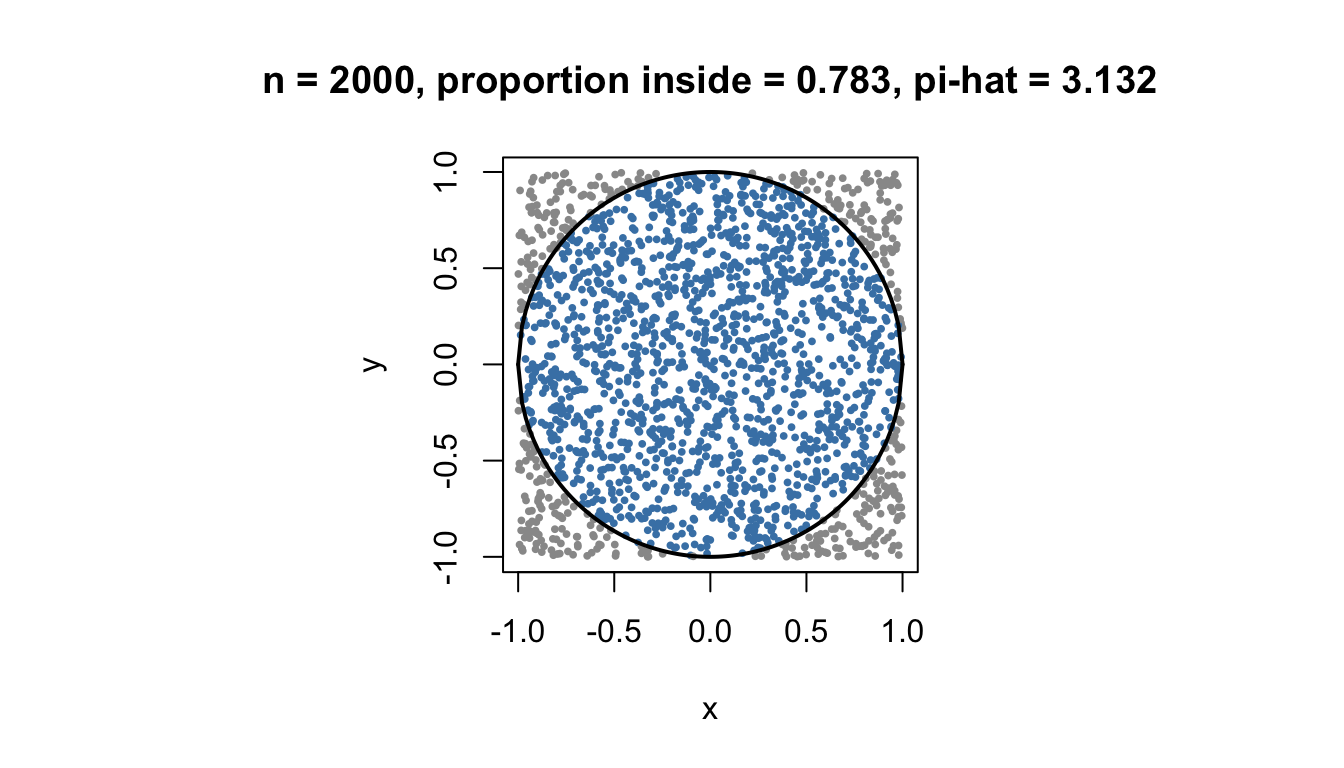
An Example: Estimating \pi by Monte Carlo
Let (X, Y) be uniform on the square S = (-1,1)\times(-1,1), and let C = \{(x,y): x^2 + y^2 \le 1\} be the unit disk. Then.
P\big((X,Y) \in C\big) = \frac{\text{area}(C)}{\text{area}(S)} = \frac{\pi}{4}.
Define Z = 4\, I\big((X,Y)\in C\big), so E(Z) = \pi and
\mathrm{Var}(Z) = 16 \cdot \frac{\pi}{4}\left(1 - \frac{\pi}{4}\right) \approx 2.70, \qquad \mathrm{SD}(Z) \approx 1.64 .
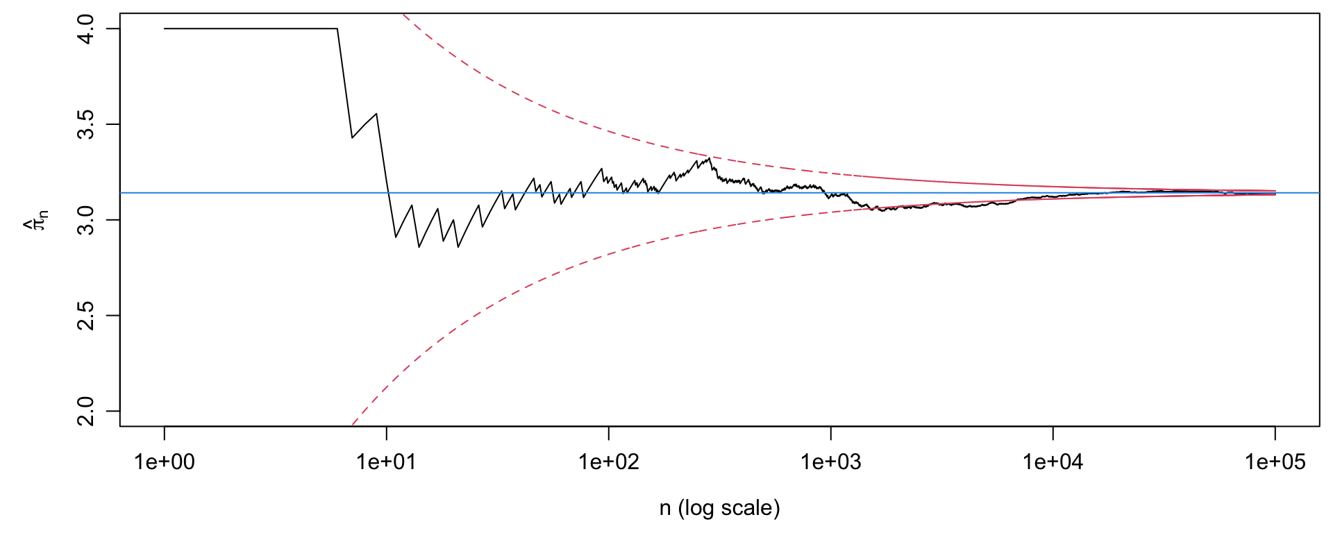
The observed error is typically within about 2 standard errors.
SE shrinks by \sqrt{10} \approx 3.2 for each 10-fold increase in n, as the CLT predicts.
Convergence of \hat\pi_n
set.seed(1)n <-1e5; z <-4* (runif(n, -1, 1)^2+runif(n, -1, 1)^2<=1)k <-1:n; pihat <-cumsum(z) / kpar(mar =c(4, 4.5, 0.5, 0.5), mgp =c(2.5, 0.8, 0))plot(k, pihat, type ="l", log ="x", ylim =c(2, 4),xlab ="n (log scale)", ylab =expression(hat(pi)[n]))lines(k, pi +1.96*1.64/sqrt(k), lty =2, col =2)lines(k, pi -1.96*1.64/sqrt(k), lty =2, col =2)abline(h = pi, col =4)
The red band is \pi \pm 1.96\,\sigma/\sqrt n; the running estimate stays inside it most of the time.
3 Evaluating a Point Estimator by Simulation
Point Estimators
A point estimator \hat\theta = \hat\theta(X_1, \ldots, X_n) is judged by its mean squared error
\mathrm{MSE}(\hat\theta) = E\big[(\hat\theta - \theta)^2\big] = \mathrm{Var}(\hat\theta) + \big[\mathrm{Bias}(\hat\theta)\big]^2 .
MSE is an expectation, so it is estimated by Monte Carlo: simulate N independent data sets from a model with known\theta,
\hat\theta^{(j)} = \hat\theta\big(X_1^{(j)}, \ldots, X_n^{(j)}\big), \qquad j = 1, \ldots, N,
and compute
\widehat{\mathrm{MSE}} = \frac{1}{N}\sum_{j=1}^N \big(\hat\theta^{(j)} - \theta\big)^2, \qquad
\widehat{\mathrm{Bias}} = \overline{\hat\theta} - \theta, \qquad
\widehat{\mathrm{Var}} = \frac{1}{N}\sum_{j=1}^N \big(\hat\theta^{(j)} - \overline{\hat\theta}\big)^2 .
Two sample sizes appear: n (data per replicate, fixed by the problem) and N (replicates, chosen large enough that the Monte Carlo error is negligible).
Example: Mean vs. Median vs. Trimmed Mean
Estimating the centre \theta = 0 of a symmetric distribution, n = 20, N = 5000 replicates.
eval_est <-function(rdist, n =20, N =5000) { est <-replicate(N, { x <-rdist(n); c(mean =mean(x), median =median(x), trim10 =mean(x, trim =0.1)) })rbind(bias =rowMeans(est), var =apply(est, 1, var), mse =rowMeans(est^2))}round(eval_est(rnorm), 4) # normal data
       mean median trim10
bias 0.0010 0.0019 0.0013
var  0.0489 0.0738 0.0514
mse  0.0489 0.0738 0.0514
round(eval_est(function(n) rt(n, df =3)), 4) # heavy-tailed t3 data
        mean  median  trim10
bias -0.0089 -0.0031 -0.0040
var   0.1438  0.0912  0.0847
mse   0.1438  0.0912  0.0847
No estimator is best everywhere: the mean wins under normality, the trimmed mean and median win under heavy tails.
4 Evaluating and Conducting Hypothesis Tests
Hypothesis Tests and the Two Types of Error
A test rejects H_0 when a statistic T exceeds a critical value c_\alpha.
\widehat{\text{FPR}} estimates the size (type I error rate); \widehat{\text{TPR}} estimates the power, 1 - \beta.
To get size \alpha, take \hat c_\alpha = the (1-\alpha) sample quantile of T^{(1)}_{H_0}, \ldots, T^{(N)}_{H_0}, which replaces the (often unknown) null distribution of T by its empirical distribution.
P-value: A PIT transfromation of T under H_0
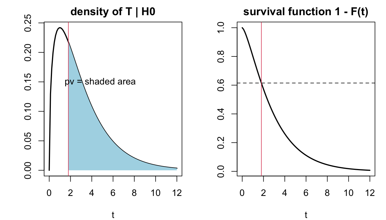
The p-value is the probability, under H_0, of a statistic at least as extreme as the observed one:
\text{p-value}(t) = P(T \ge t \mid H_0) = 1 - F_{H_0}(t),
the survival function of T under H_0 evaluated at t^{obs}. Rejecting when \text{p-value}(t^{obs}) < \alpha is the same as rejecting when t^{obs} > c_\alpha.
Uniformity of \text{p-value}(T) under H_0
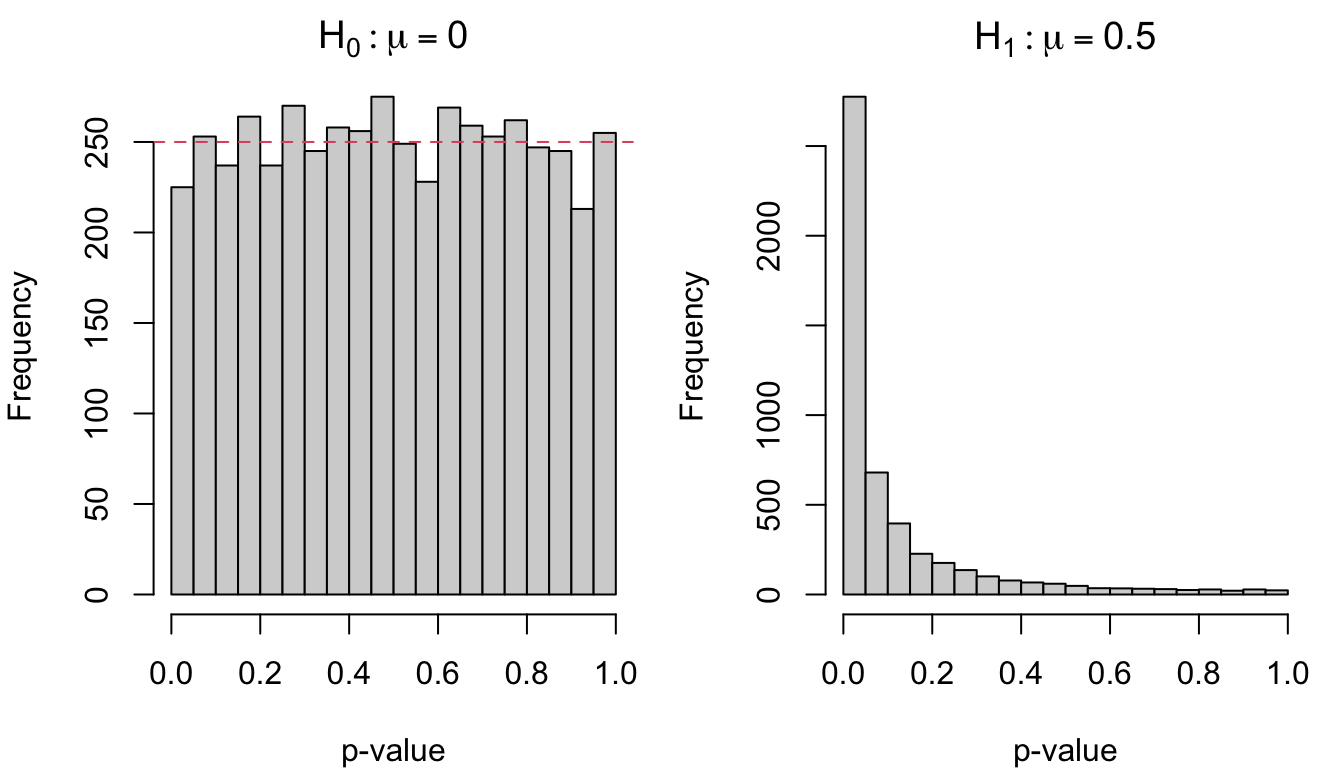
Theorem. If T \mid H_0 has continuous CDF F_{H_0}, then \text{p-value}(T) = 1 - F_{H_0}(T) \sim \mathrm{Unif}(0,1) under H_0.
c(size =mean(pv0 <0.05), power =mean(pv1 <0.05),exact_power =power.t.test(n =20, delta =0.5, sd =1, type ="one.sample")$power)
       size       power exact_power
  0.0450000   0.5550000   0.5644829
Each estimate is a proportion, so its Monte Carlo standard error is \sqrt{\hat p(1-\hat p)/N} — about 0.003 for the size with N = 5000.
Monte Carlo for Calculating (Not Evaluating) a P-value
When F_{H_0} is unknown, estimate \text{p-value}(t^{obs}) by simulating T under H_0:
\widehat{\text{p-value}}(t^{obs}) = \frac{1 + \sum_{j=1}^N I\big(T^{(j)} \ge t^{obs}\big)}{N + 1}.
(The “+1” counts the observed statistic as one draw from H_0; it keeps the estimate above 0 and the test exactly valid.)
Example: test H_0: \mu = 0 for n = 15 observations using T = \lvert\overline X
\rvert/(s/\sqrt n), but suppose we did not know the t-distribution.
x <-rnorm(15, mean =0.6); tobs <-abs(mean(x)) / (sd(x) /sqrt(15))Tnull <-replicate(5000, { y <-rnorm(15); abs(mean(y)) / (sd(y) /sqrt(15)) })c(mc_pv = (1+sum(Tnull >= tobs)) /5001, exact_pv =2*pt(-tobs, df =14))
     mc_pv   exact_pv
0.08518296 0.07933636
Example 1: A Permutation Test for the Correlation Coefficient
Setting and Procedure
Data (X_i, Y_i), i = 1, \ldots, n. Test H_0: X \perp Y (which implies \mathrm{corr}(X,Y) = 0) with T = \lvert\hat\rho
\rvert.
Under H_0, every pairing of the X values with the Y values is equally likely, so the null distribution of T is obtained by re-computing T after randomly permuting Y:
Compute \rho^{obs} = \hat\rho(X, Y).
For j = 1, \ldots, m: permute Y to get Y^{(j)}, compute \rho^{(j)} = \hat\rho(X, Y^{(j)}).
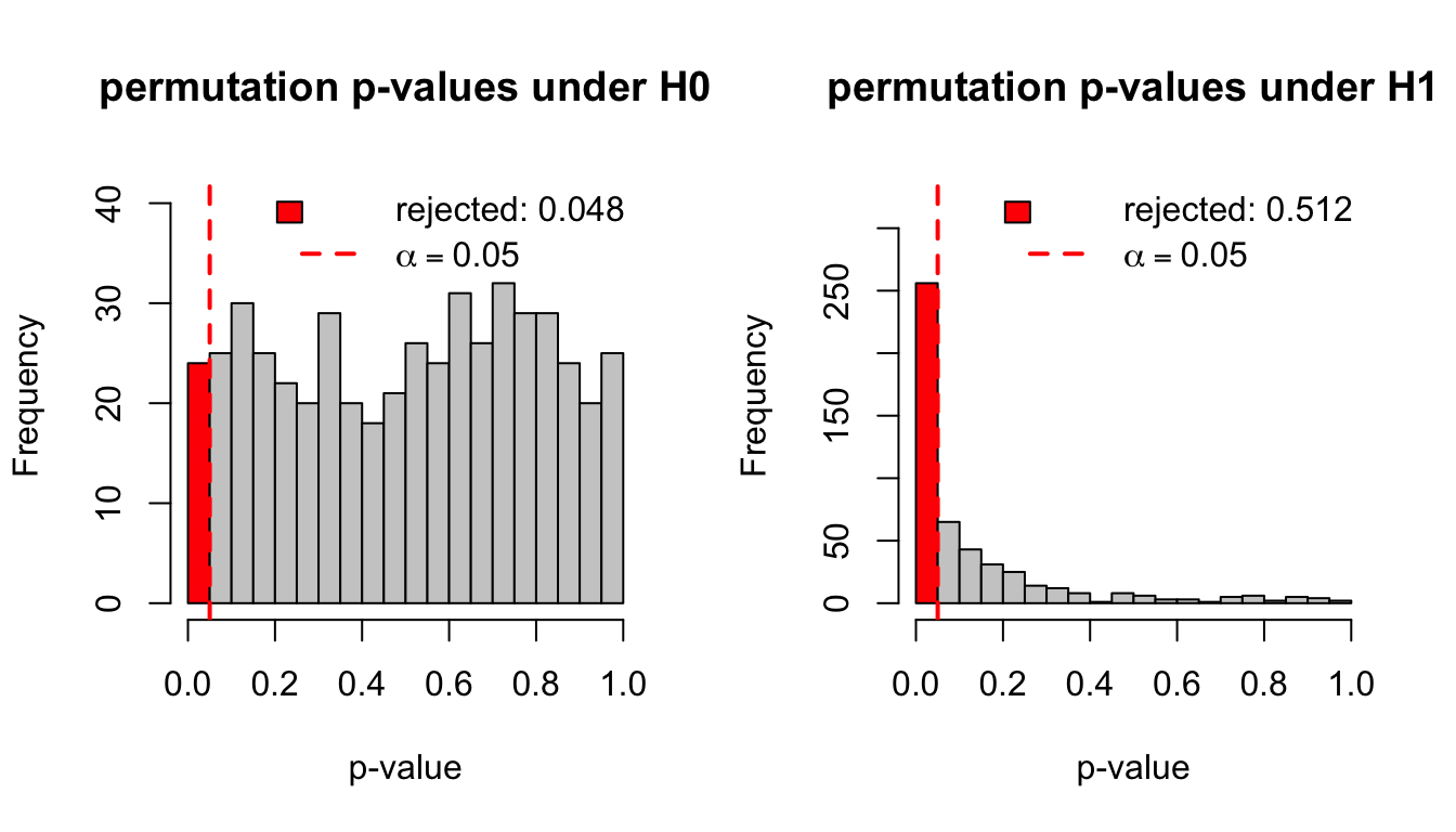
Generate non-normal (X, Y): independent under H_0, and Y = 0.4X + \epsilon under H_1. Check that the permutation p-values are uniform with size \alpha under H_0, and estimate the power under H_1.
sim_cor <-function(n =30, b =0) { x <-rexp(n); list(x = x, y = b * x +rexp(n)) }eval_perm_cor <-function(b, N =500) replicate(N, { d <-sim_cor(b = b)perm_cor_test(d$x, d$y, m =500)$pv})pv_cor0 <-eval_perm_cor(b =0) # H0: independentpv_cor1 <-eval_perm_cor(b =0.4) # H1: dependenthist_reject <-function(pv, main, alpha =0.05) { br <-seq(0, 1, by = alpha) # first bar = rejection region ymax <-max(hist(pv, breaks = br, plot =FALSE)$counts)hist(pv, breaks = br, main = main, xlab ="p-value",ylim =c(0, 1.3* ymax), # headroom for the legendcol =ifelse(br[-1] <= alpha, "red", "grey80"))abline(v = alpha, col ="red", lwd =2, lty =2)legend("topright", bty ="n", fill =c("red", NA), border =c("black", NA),lty =c(NA, 2), col =c(NA, "red"), lwd =c(NA, 2),legend =c(sprintf("rejected: %.3f", mean(pv < alpha)),as.expression(bquote(alpha == .(alpha)))))}par(mfrow =c(1, 2))hist_reject(pv_cor0, "permutation p-values under H0")hist_reject(pv_cor1, "permutation p-values under H1")
Under H_0 the permutation p-values are uniform on [0,1] and the size is close to 0.05, with no distributional assumption on (X, Y). Under H_1 they pile up near 0; the proportion below 0.05 is the power.
Example 2: Testing for Post-selection Regression
Setting
Response Y and p = 20 candidate predictors X_1, \ldots, X_{20}, n = 50. We want to test H_0: Y is unrelated to all of the X’s.
A common practice:
Pick the predictor X_{k^*} most correlated with Y.
Fit Y \sim X_{k^*} and report the usual t-test p-value for its slope.
Question. Is this a valid test of H_0? Does it have size \alpha?
A Test With Post-Selection Fitting
test_lm_sel <-function(y, X) { k <-which.max(abs(cor(X, y)))summary(lm(y ~ X[, k]))$coefficients[2, 4] # t-test p-value of selected slope}
The t-test p-value assumes X_{k^*} was chosen in advance. Selecting the best of 20 predictors after looking at the data means that, even under H_0, \max_k \lvert\hat\rho_k
\rvert tends to be large. The reported p-value ignores this selection.
Simulation for Evaluating test_lm_sel
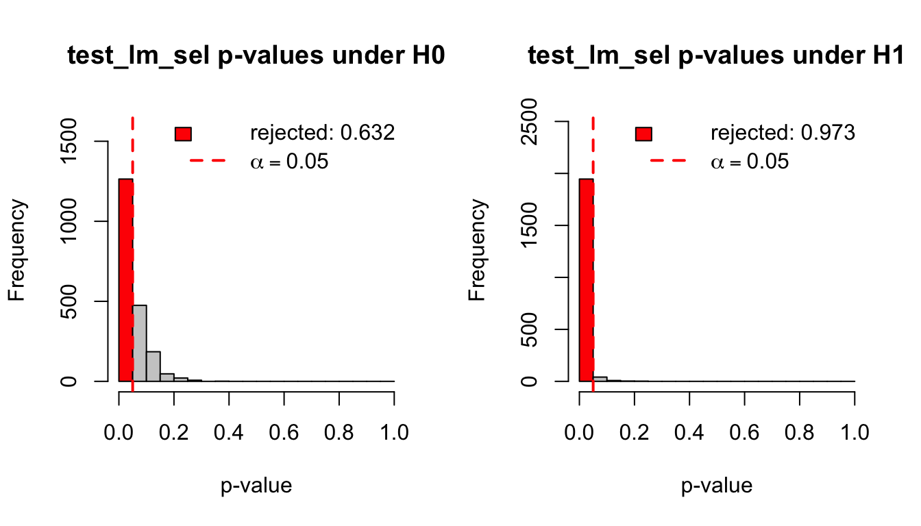
Simulate N = 2000 datasets with Y = \beta X_1 + \epsilon: \beta = 0 under H_0, and \beta = 0.5 under H_1.
sim_lm <-function(n =50, p =20, beta =0) { X <-matrix(rnorm(n * p), n, p); list(y = beta * X[, 1] +rnorm(n), X = X)}pv_sel0 <-replicate(2000, { d <-sim_lm(beta =0); test_lm_sel(d$y, d$X) })pv_sel1 <-replicate(2000, { d <-sim_lm(beta =0.5); test_lm_sel(d$y, d$X) })par(mfrow =c(1, 2))hist_reject(pv_sel0, "test_lm_sel p-values under H0")hist_reject(pv_sel1, "test_lm_sel p-values under H1")
The true size is far above 0.05: test_lm_sel rejects a true H_0 far too often. Under H_0 its p-value is not uniform, which is a general diagnostic for an invalid test. Its high rejection rate under H_1 is not real power, since the test does not have size \alpha.
Permutation Test for Post-selection Regression
Fix: repeat the whole procedure — select the most correlated variable, fit the linear model, report its p-value — on permuted responses, and compare the observed p-value with the permutation distribution of p-values.
Compute p^{obs} = p-value of test_lm_sel on (Y, X).
For j = 1, \ldots, m: permute Y, compute p^{(j)} = p-value of test_lm_sel on (Y^{(j)}, X) (re-doing the selection each time).
\widehat{\text{p-value}} = \dfrac{1 + \# \{j : p^{(j)} \le p^{obs}\}}{m+1}, the proportion of permuted p-values at least as small as the observed one.
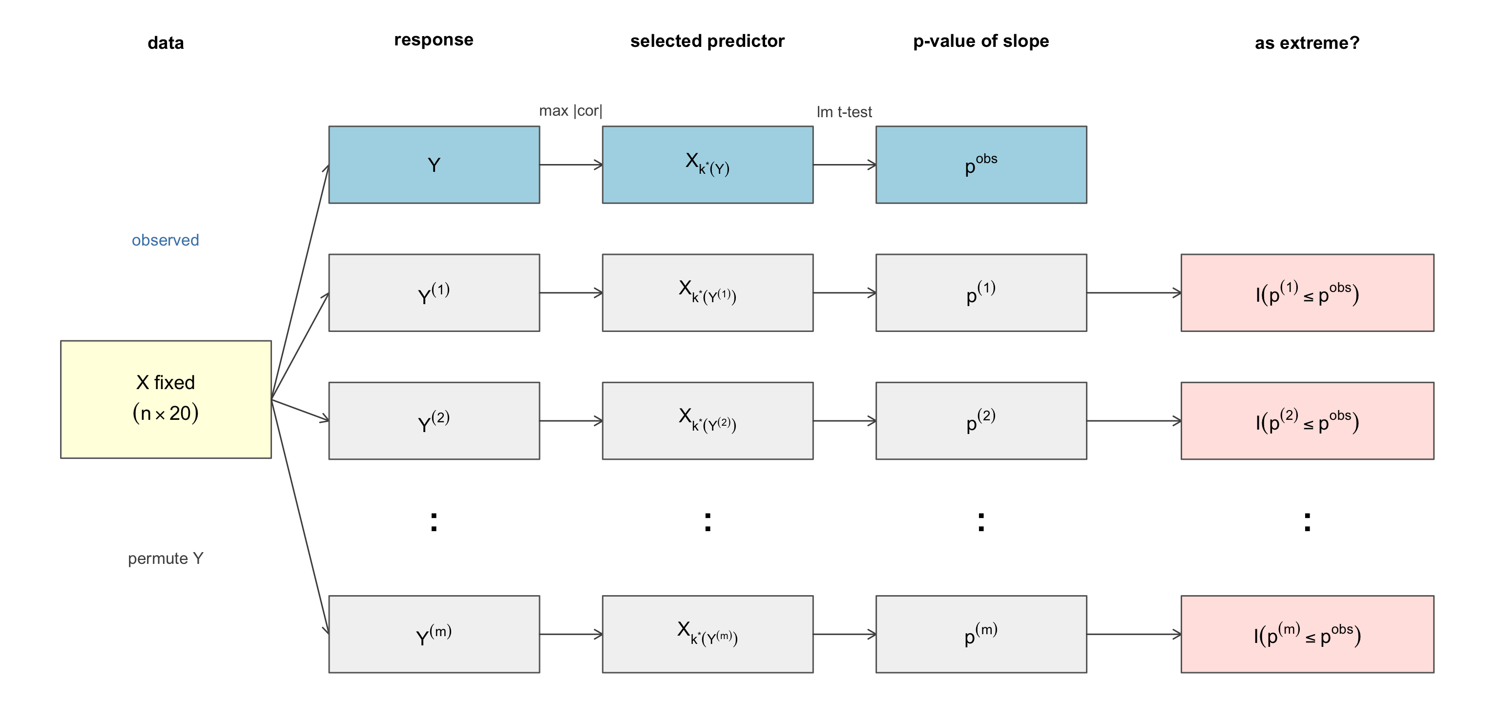
Tree Diagram: Re-selecting the Predictor with Permuated Y
k^*(Y) = \arg\max_k \lvert\hat\rho(X_k, Y)\rvert is the index of the column of X most correlated with the response. It is a function of the response, so each permuted Y^{(j)} gets its own selected predictor X_{k^*(Y^{(j)})}:
Keeping X_{k^*(Y)} fixed and only permuting Y would not reproduce the selection step, and the resulting test would still be invalid.
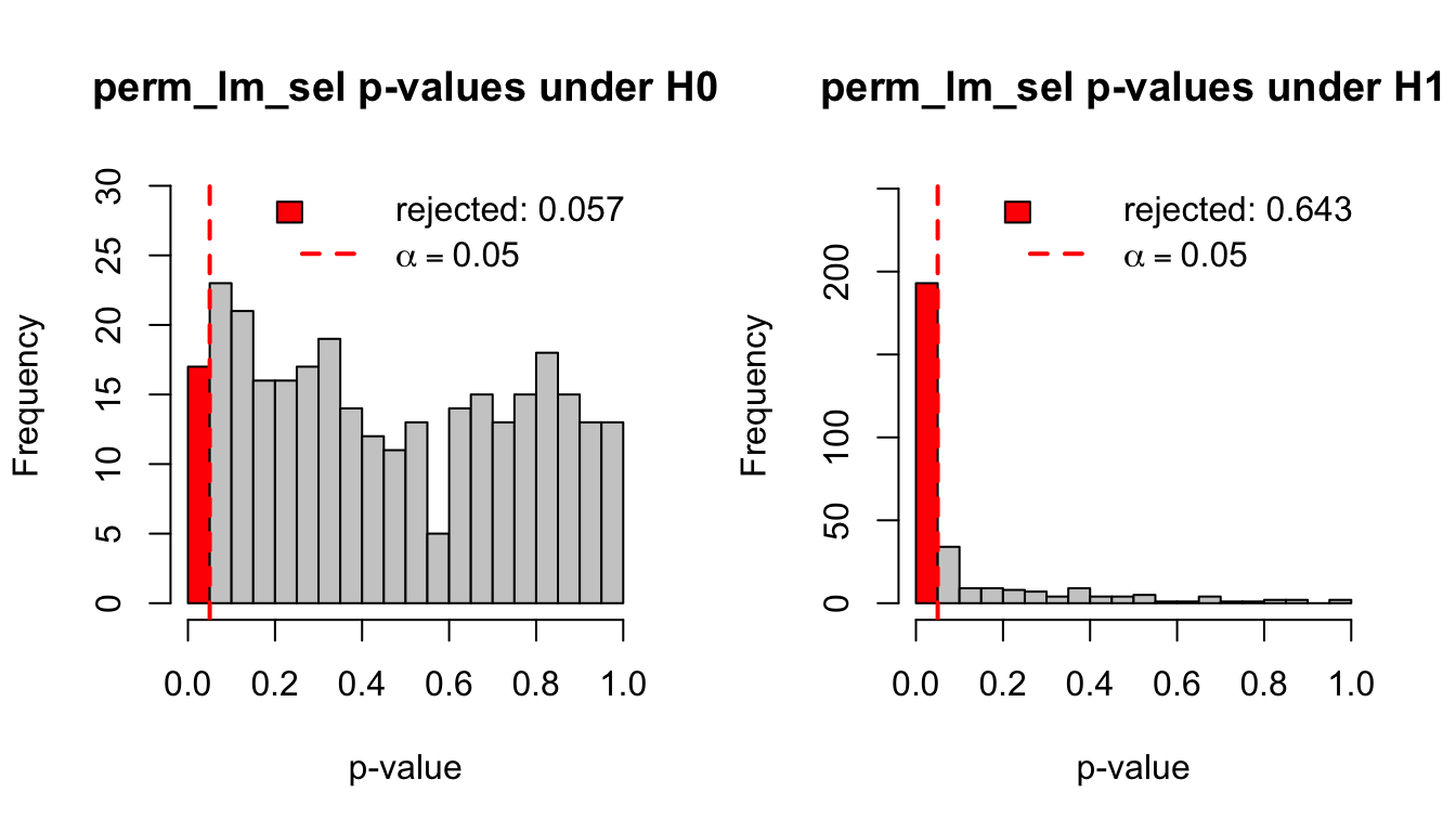
Simulate (Y, X) from sim_lm: \beta = 0 under H_0, and \beta = 0.5 under H_1. Check that the permutation p-values are uniform with size \alpha under H_0, and estimate the power under H_1.
eval_perm_lm_sel <-function(beta, N =300) replicate(N, { d <-sim_lm(beta = beta)perm_lm_sel(d$y, d$X, m =500)})pv_perm0 <-eval_perm_lm_sel(beta =0) # H0: Y unrelated to Xpv_perm1 <-eval_perm_lm_sel(beta =0.5) # H1: Y depends on X1par(mfrow =c(1, 2))hist_reject(pv_perm0, "perm_lm_sel p-values under H0")hist_reject(pv_perm1, "perm_lm_sel p-values under H1")
Under H_0 the permutation p-values are uniform and the size is close to 0.05; under H_1 they pile up near 0, and the proportion below 0.05 is an honest power.
Summary
All simulation starts from pseudo-random \mathrm{Unif}(0,1) draws; other distributions come from inverse-CDF or transformations (Box–Muller).
The LLN justifies Monte Carlo averages; the CLT gives their error, \sigma/\sqrt n, which is reported as a standard error.
Bias, variance and MSE of estimators, and size and power of tests, are expectations — simulate with known truth and average.
P-values are uniform under H_0: a flat histogram of simulated p-values is the basic test of a test.
When the null distribution is unknown, generate it by simulation or by permutation; the permuted statistic must reproduce the entire data-analysis procedure.