Elements of Statistical Computation

Optimization for Maximum Likelihood Estimation

Longhai Li

2026-10-06

1 Review: Likelihood Theory and MLE

Likelihood Function

A statistical model specifies the probability (density) of data D given a parameter \theta: f(D \mid \theta).

• As a function of D for fixed \theta: the sampling distribution.

• As a function of \theta for fixed (observed) D: the likelihood function. L(\theta; D) = f(D \mid \theta).

The likelihood measures how well each value of \theta explains the observed data. For iid data D = (x_1, \ldots, x_n), L(\theta; D) = \prod_{i=1}^n f(x_i \mid \theta), \qquad \ell(\theta) = \log L(\theta; D) = \sum_{i=1}^n \log f(x_i \mid \theta).

We work with the log-likelihood \ell(\theta) to avoid underflow of the product and because sums are easier to differentiate.

Maximum Likelihood (Minimum Loss) Estimator

\hat\theta_{\mathrm{MLE}} = \arg\max_\theta L(\theta; D) = \arg\max_\theta \ell(\theta) = \arg\min_\theta \mathcal{L}(\theta), \qquad \mathcal{L}(\theta) = -\ell(\theta).

Every algorithm in this lecture minimizes the negative log-likelihood \mathcal{L} (nll in code). Three quantities recur:

• the gradient g(\theta) = \mathcal{L}'(\theta) = -\ell'(\theta), whose root locates the minimum;
• the observed information J(\theta) = g'(\theta) = \mathcal{L}''(\theta) = -\ell''(\theta);
• the expected information nI(\theta) = E_D[\,g'(\theta; D)\,].

The classical score is \ell'(\theta) = -g(\theta); we work with g throughout so that every method is a minimization.

Example: Bernoulli Likelihood

Y_1, Y_2, Y_3 \overset{iid}{\sim} \mathrm{Bern}(\theta), observed y = (1, 1, 0).

\theta	P(1, 1, 0 \mid \theta) = \theta^2(1-\theta)
0	0
1/2	1/8 = 0.1250
2/3	4/27 = 0.1481 (max)
3/4	9/64 = 0.1406
1	0

Example: Bernoulli Likelihood

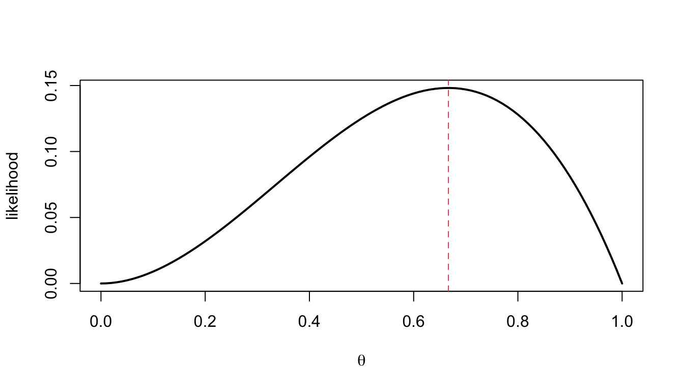
P(y_i \mid \theta) = \theta^{y_i}(1-\theta)^{1-y_i}, so with n_1 = \sum y_i and n_0 = n - n_1, L(\theta) = \theta^{n_1}(1-\theta)^{n_0}, \qquad \ell(\theta) = n_1\log\theta + n_0\log(1-\theta).

The negative log-likelihood and its gradient are \mathcal{L}(\theta) = -n_1\log\theta - n_0\log(1-\theta), \qquad g(\theta) = \mathcal{L}'(\theta) = \frac{n_0}{1-\theta} - \frac{n_1}{\theta} .

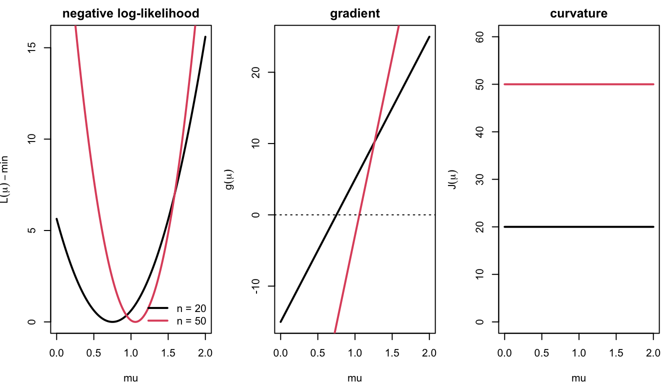
The MLE solves g(\theta) = 0 \iff \hat\theta = \dfrac{n_1}{n} = \overline y, and the curvature J(\theta) = g'(\theta) = \dfrac{n_1}{\theta^2} + \dfrac{n_0}{(1-\theta)^2} > 0 confirms a minimum of \mathcal{L}.

Example: Normal Mean with Known Variance

X_1, \ldots, X_n \overset{iid}{\sim} N(\mu, \sigma_0^2): \mathcal{L}(\mu) = \frac{n}{2}\log(2\pi\sigma_0^2) + \frac{1}{2\sigma_0^2}\sum_{i=1}^n (x_i - \mu)^2 = C + \frac{n}{2\sigma_0^2}(\mu - \overline x)^2, using \sum(x_i - \mu)^2 = \sum(x_i - \overline x)^2 + n(\overline x - \mu)^2. g(\mu) = \frac{n}{\sigma_0^2}(\mu - \overline x) = 0 \implies \hat\mu = \overline x, \qquad J(\mu) = g'(\mu) = \frac{n}{\sigma_0^2}.

• \mathcal{L} is exactly quadratic in \mu; the gradient g is linear; the curvature J is constant and grows with n.

• J = \mathcal{L}'' = -\ell'' measures how sharply the data pin down \mu: it is the Fisher information.

Negative Log-likelihood, Gradient and Curvature

The gradient crosses zero where \mathcal{L} is minimized; larger n makes \mathcal{L} more sharply curved, g steeper, and J larger.

Example: Cauchy Location

X_1, \ldots, X_n \overset{iid}{\sim} \mathrm{Cauchy}(\theta), f(x \mid \theta) = \dfrac{1}{\pi\,[1 + (x-\theta)^2]}: \mathcal{L}(\theta) = n\log\pi + \sum_{i=1}^n \log\!\big(1 + (x_i - \theta)^2\big), \qquad g(\theta) = \sum_{i=1}^n \frac{2(\theta - x_i)}{1 + (x_i - \theta)^2}.

The equation g(\theta) = 0 has no closed-form solution and may have several roots:

xc <- rcauchy(8, location = 3)
nllc <- function(th, dat) sapply(th, function(t) -sum(dcauchy(dat, t, log = TRUE)))
curve(nllc(x, xc), -10, 15, lwd = 2, xlab = expression(theta), ylab = expression(L(theta)), main = "Cauchy negative log-likelihood, n = 8")

This is why we need numerical optimization.

Properties of the MLE

Under regularity conditions (satisfied by most models in practice), for iid data with true parameter \theta_*:

1. Consistency: \hat\theta_{\mathrm{MLE}} \to \theta_* as n \to \infty.

2. Asymptotic normality: \hat\theta_{\mathrm{MLE}} \;\dot\sim\; N\!\big(\theta_*,\ [n I(\theta_*)]^{-1}\big), \qquad I(\theta) = -E_X\!\left[\frac{\partial^2}{\partial\theta\,\partial\theta'}\log f(X \mid \theta)\right], the expected Fisher information per observation (p \times p for a p-dimensional \theta).

3. Asymptotic efficiency: no consistent estimator has smaller asymptotic variance (Cramér–Rao bound).

Note n I(\theta) = E_D\big[\mathcal{L}''(\theta; D)\big] = -E_D\big[\ell''(\theta; D)\big]: the expected curvature of \mathcal{L}.

Observed and Expected Fisher Information

\theta_* is unknown, so the variance [nI(\theta_*)]^{-1} is estimated by plugging in \hat\theta. Two versions:

• Expected information n I(\hat\theta): requires computing E_X[\cdot] analytically.

• Observed information J(\hat\theta) = \mathcal{L}''(\hat\theta; D) = g'(\hat\theta) = -\sum_{i=1}^n \frac{\partial^2}{\partial\theta\partial\theta'}\log f(x_i \mid \hat\theta): the actual curvature at the MLE, no expectation needed.

By the LLN, J(\hat\theta)/n \approx I(\hat\theta). Both give \widehat{\mathrm{Var}}(\hat\theta) \approx J(\hat\theta)^{-1} \quad\text{or}\quad [nI(\hat\theta)]^{-1}, \qquad \widehat{\mathrm{SE}}(\hat\theta_j) = \sqrt{\big[\widehat{\mathrm{Var}}(\hat\theta)\big]_{jj}} .

Computational consequence: the Hessian of \mathcal{L} at the optimum, which Newton-type optimizers compute anyway, gives the standard errors for free.

2 Univariate Optimization

The Problem

Minimize \mathcal{L}(\theta) = -\ell(\theta), \theta \in \mathbb{R}; equivalently, find a root of g(\theta) = \mathcal{L}'(\theta), or rearrange that root equation into a fixed point \theta = \varphi(\theta).

Methods differ in what they need and how fast they converge:

method	needs	convergence
fixed-point iteration	a rearrangement \theta = \varphi(\theta)	linear, if at all
bisection	g(\theta) and a sign-changing bracket	linear (halves bracket)
golden section	\mathcal{L}(\theta) only, and a bracket	linear
Newton–Raphson	g(\theta) and g'(\theta) = \mathcal{L}''(\theta)	quadratic near root
Fisher scoring	g(\theta) and I(\theta)	linear–quadratic

Every method below is illustrated on the same zero-truncated Poisson likelihood, so the pictures are directly comparable.

Running Example: Zero-Truncated Poisson

We observe only the nonzero counts of a Poisson process (X = Y \mid Y > 0, Y \sim \mathrm{Pois}(\lambda)): P(x \mid \lambda) = \frac{e^{-\lambda}\lambda^x}{x!}\cdot\frac{1}{1 - e^{-\lambda}}, \qquad x = 1, 2, \ldots \mathcal{L}(\lambda) = n\lambda - \sum x_i \log\lambda + n\log(1 - e^{-\lambda}) + C g(\lambda) = \frac{n}{1 - e^{-\lambda}} - \frac{\sum x_i}{\lambda} g'(\lambda) = \frac{\sum x_i}{\lambda^2} - \frac{n e^{-\lambda}}{(1 - e^{-\lambda})^2}.

Using E(X) = \dfrac{\lambda}{1 - e^{-\lambda}}, nI(\lambda) = E[g'(\lambda)] = \frac{n}{\lambda(1 - e^{-\lambda})} - \frac{n e^{-\lambda}}{(1 - e^{-\lambda})^2}.

Zero-Truncated Poisson in R

library(latex2exp)
set.seed(812)
y <- rpois(200, 1.5); x <- y[y > 0]; n <- length(x); sx <- sum(x); xbar <- mean(x)
nll <- function(l) n * l - sx * log(l) + n * log(1 - exp(-l))   # the objective
g   <- function(l) n / (1 - exp(-l)) - sx / l                   # gradient  L'(lambda)
dg  <- function(l) sx / l^2 - n * exp(-l) / (1 - exp(-l))^2     # curvature L''(lambda)
nI  <- function(l) n / (l * (1 - exp(-l))) - n * exp(-l) / (1 - exp(-l))^2
lhat <- uniroot(g, c(1e-6, 20), tol = 1e-12)$root   # reference value for the pictures
lam  <- seq(0.4, 4, length.out = 400)               # plotting grid used throughout
c(naive_mean = xbar, mle = lhat, true_lambda = 1.5)

 naive_mean         mle true_lambda 
   1.920000    1.485204    1.500000 

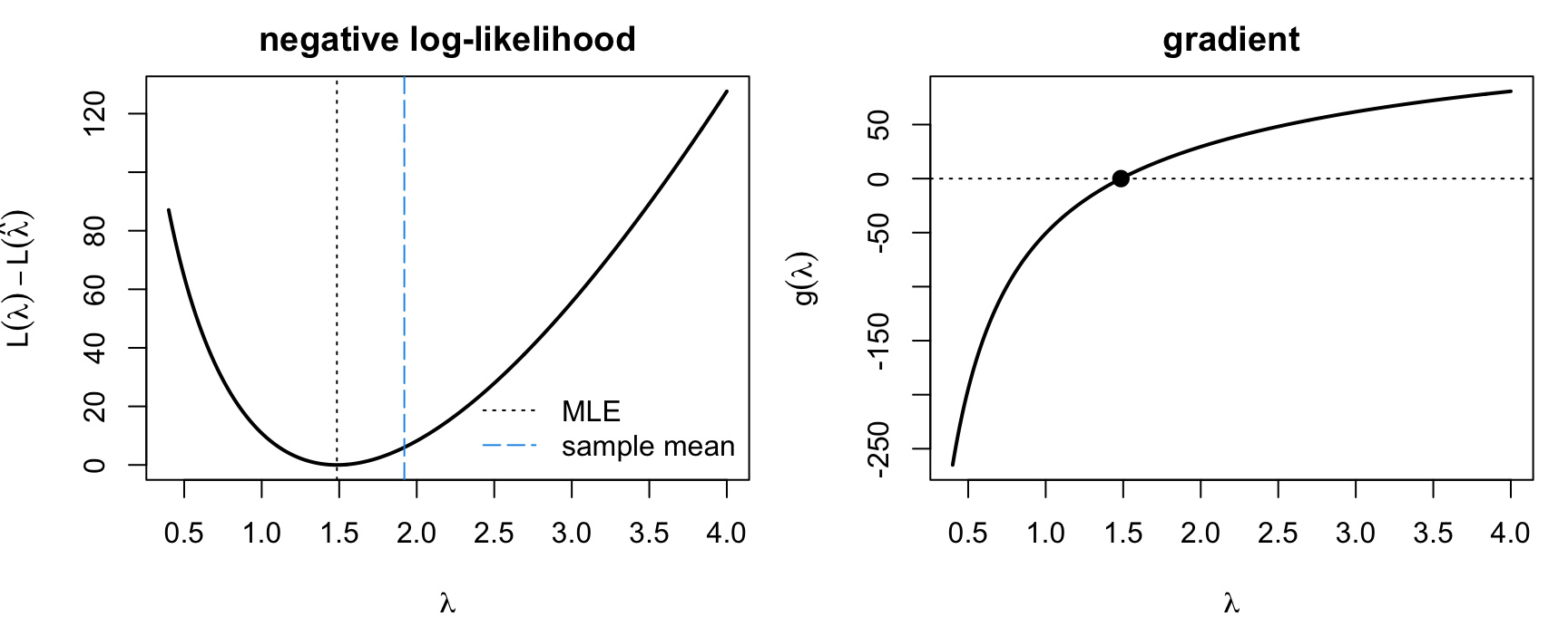
par(mfrow = c(1, 2), mar = c(4.2, 4.2, 2.2, 1))
plot(lam, nll(lam) - nll(lhat), type = "l", lwd = 2, main = "negative log-likelihood",
     xlab = TeX("$\\lambda$"), ylab = TeX("$L(\\lambda) - L(\\hat{\\lambda})$"))
abline(v = lhat, lty = 3); abline(v = xbar, col = 4, lty = 5)
legend("bottomright", bty = "n", lty = c(3, 5), col = c(1, 4), legend = c("MLE", "sample mean"))
plot(lam, g(lam), type = "l", lwd = 2, main = "gradient",
     xlab = TeX("$\\lambda$"), ylab = TeX("$g(\\lambda)$"))
abline(h = 0, lty = 3); points(lhat, 0, pch = 19, cex = 1.2)

The plain sample mean overestimates \lambda because the zeros are missing; the MLE sits where the gradient crosses zero.

Fixed-Point Iteration: Two Rearrangements

The stationarity equation g(\lambda) = 0 can be written as \frac{\overline x}{\lambda} = \frac{1}{1 - e^{-\lambda}} .

Solving for the \lambda on the left gives one rearrangement; solving for the exponential gives another: \lambda = \overline x\,(1 - e^{-\lambda}) =: \varphi_1(\lambda), \qquad \lambda = -\log\!\Big(1 - \frac{\lambda}{\overline x}\Big) =: \varphi_2(\lambda) .

Both have exactly the same fixed points, \hat\lambda and the spurious root \lambda = 0, and indeed \varphi_2 = \varphi_1^{-1}. (The map is written \varphi, not g, because g is reserved for the gradient.)

Fixed-Point Iteration: The Method

Pick a rearrangement \lambda = \varphi(\lambda) and iterate \lambda_{k+1} = \varphi(\lambda_k), \qquad k = 0, 1, 2, \ldots

Writing e_k = \lambda_k - \lambda^* and expanding \varphi about the fixed point, e_{k+1} \approx \varphi'(\lambda^*) e_k:

• the iteration converges to \lambda^* when |\varphi'(\lambda^*)| < 1, and the error then shrinks by that constant factor each step — linear convergence;
• it is repelled from \lambda^* when |\varphi'(\lambda^*)| > 1.

Here \varphi_1'(\lambda) = \overline x\, e^{-\lambda} and \varphi_2'(\lambda) = (\overline x - \lambda)^{-1}. Since \varphi_2 = \varphi_1^{-1}, the slopes are reciprocal at every fixed point, so at most one of the two rearrangements can converge to \hat\lambda.

fixed_point <- function(phi, x0, tol = 1e-8, maxit = 500) {
  for (k in 1:maxit) { x1 <- phi(x0); if (abs(x1 - x0) < tol) return(c(root = x1, iter = k)); x0 <- x1 }
  stop("not converged")
}
phi1 <- function(l) xbar * (1 - exp(-l))
phi2 <- function(l) -log(1 - l / xbar)
fixed_point(phi1, x0 = xbar)

     root      iter 
 1.485204 22.000000 

Advantage: no derivatives. Disadvantage: a suitable \varphi must be found, and the rearrangement alone decides the outcome.

Fixed-Point: The Cobweb

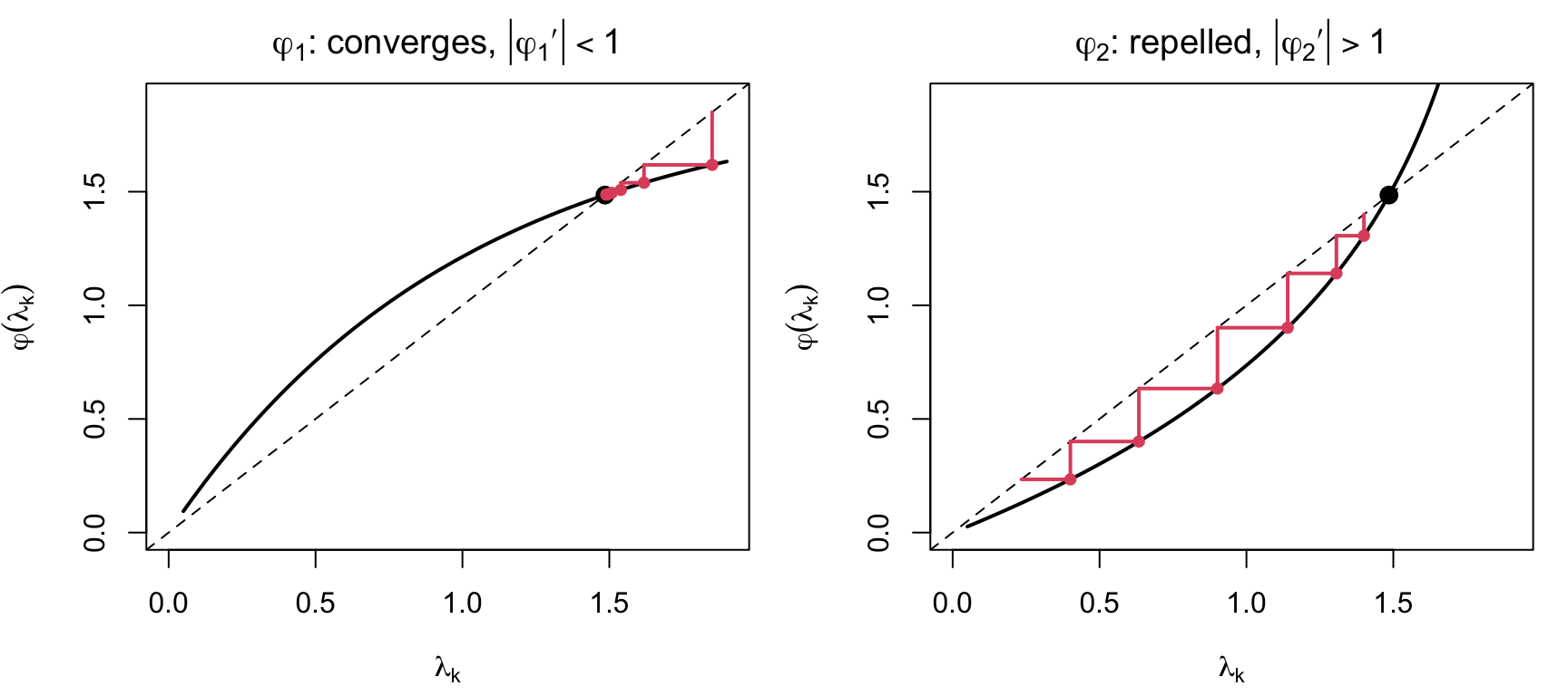
cobweb <- function(phi, x0, nstep, main) {
  gg <- seq(0.05, 1.9, length.out = 300)
  plot(gg, phi(gg), type = "l", lwd = 2, xlim = c(0, 1.9), ylim = c(0, 1.9),
       xlab = TeX("$\\lambda_k$"), ylab = TeX("$\\varphi(\\lambda_k)$"), main = main)
  abline(0, 1, lty = 2); points(lhat, lhat, pch = 19, cex = 1.3)
  for (k in 1:nstep) {
    x1 <- phi(x0); if (!is.finite(x1) || x1 < 0) break
    segments(x0, x0, x0, x1, col = 2, lwd = 2)     # up (or down) to the curve
    segments(x0, x1, x1, x1, col = 2, lwd = 2)     # across to the diagonal
    points(x0, x1, pch = 19, col = 2, cex = 0.8)
    x0 <- x1
  }
}
par(mfrow = c(1, 2), mar = c(4.2, 4.2, 2.4, 1))
cobweb(phi1, x0 = 1.85, nstep = 6, main = TeX("$\\varphi_1$: converges, $|\\varphi_1'| < 1$"))
cobweb(phi2, x0 = 1.40, nstep = 6, main = TeX("$\\varphi_2$: repelled, $|\\varphi_2'| > 1$"))

The staircase walks to the intersection of \varphi with the 45^\circ line. For \varphi_1 the crossing is shallow and each step strides toward it; \varphi_2 is the inverse map, its slope there is the reciprocal, and the iterates are pushed away from \hat\lambda toward the fixed point at \lambda = 0.

Fixed-Point: Traces of the Iterates

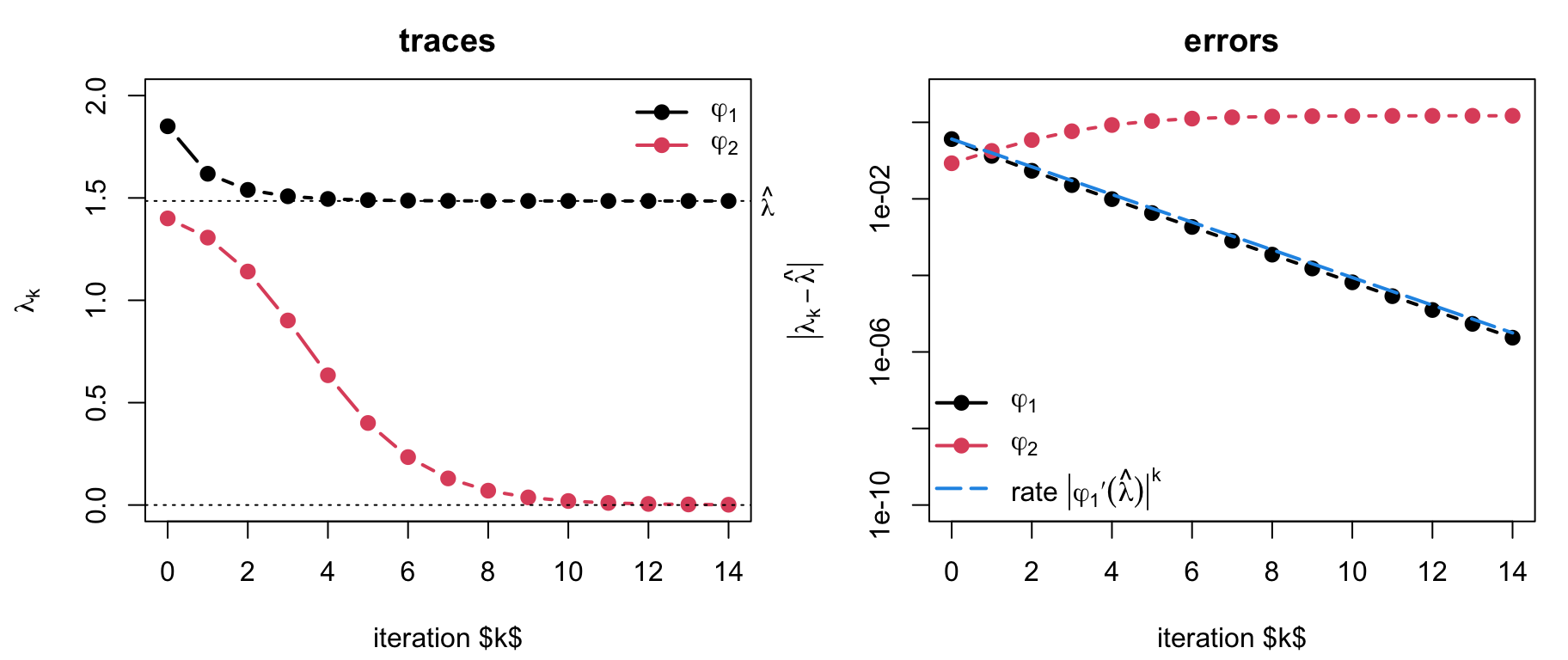
trace_fp <- function(phi, x0, nstep) {
  p <- x0
  for (k in 1:nstep) {
    xn <- phi(p[k])
    if (!is.finite(xn) || xn <= 0) break
    p <- c(p, xn)
  }
  p
}
t1 <- trace_fp(phi1, 1.85, 14); t2 <- trace_fp(phi2, 1.40, 14)
par(mfrow = c(1, 2), mar = c(4.2, 4.4, 2.4, 1))

## (a) the iterates themselves
plot(seq_along(t1) - 1, t1, type = "b", pch = 19, lwd = 2, ylim = c(0, 2),
     xlim = c(0, 14), xlab = "iteration $k$", ylab = TeX("$\\lambda_k$"), main = "traces")
lines(seq_along(t2) - 1, t2, type = "b", pch = 19, lwd = 2, col = 2)
abline(h = lhat, lty = 3); abline(h = 0, lty = 3)
mtext(TeX("$\\hat{\\lambda}$"), side = 4, at = lhat, las = 1, line = 0.3, cex = 0.9)
legend("topright", bty = "n", lwd = 2, pch = 19, col = c(1, 2),
       legend = c(TeX("$\\varphi_1$"), TeX("$\\varphi_2$")))

## (b) the errors, on a log scale
e1 <- pmax(abs(t1 - lhat), 1e-16); e2 <- pmax(abs(t2 - lhat), 1e-16)
plot(seq_along(e1) - 1, e1, type = "b", pch = 19, lwd = 2, log = "y",
     ylim = c(1e-10, 5), xlim = c(0, 14),
     xlab = "iteration $k$", ylab = TeX("$|\\lambda_k - \\hat{\\lambda}|$"), main = "errors")
lines(seq_along(e2) - 1, e2, type = "b", pch = 19, lwd = 2, col = 2)
lines(0:14, e1[1] * (xbar * exp(-lhat))^(0:14), lty = 5, col = 4, lwd = 2)
legend("bottomleft", bty = "n", lwd = 2, lty = c(1, 1, 5), pch = c(19, 19, NA),
       col = c(1, 2, 4), legend = c(TeX("$\\varphi_1$"), TeX("$\\varphi_2$"), TeX("rate $|\\varphi_1'(\\hat{\\lambda})|^k$")))

Left: \varphi_1 settles onto \hat\lambda within a few steps, while \varphi_2 slides past it and decays toward the spurious fixed point at zero. Right: the \varphi_1 error falls along a straight line on the log scale, with the slope predicted by |\varphi_1'(\hat\lambda)| — one fixed number of digits gained per iteration, against Newton’s doubling. The \varphi_2 error rises and then flattens at \hat\lambda, the distance from the limit 0 to the root it failed to find.

Bisection

If g is continuous and g(a), g(b) have opposite signs, a root lies in [a, b]. Evaluate g at the midpoint and keep the half that still brackets the root.

bisection <- function(g, a, b, tol = 1e-8) {
  k <- 0
  while (b - a > tol) { m <- (a + b) / 2; if (g(a) * g(m) <= 0) b <- m else a <- m; k <- k + 1 }
  c(root = (a + b) / 2, iter = k)
}
bisection(g, 0.1, 10)

     root      iter 
 1.485204 30.000000 

• Guaranteed to converge; the bracket halves each step, so \log_2\big((b-a)/\text{tol}\big) \approx 30 iterations here.

• Needs only g, not g'. R’s uniroot() uses a refined version (Brent’s method).

Bisection, Visualized

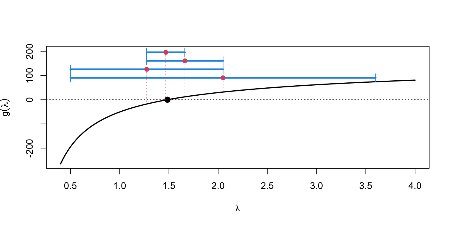
gv <- g(lam); yr <- range(gv); pad <- 0.35 * diff(yr)
plot(lam, gv, type = "l", lwd = 2, ylim = c(yr[1], yr[2] + pad),
     xlab = TeX("$\\lambda$"), ylab = TeX("$g(\\lambda)$"))
abline(h = 0, lty = 3); points(lhat, 0, pch = 19, cex = 1.3)

a <- 0.5; b <- 3.6
ylev <- seq(yr[2] + 0.08 * pad, yr[2] + 0.95 * pad, length.out = 4)
for (k in 1:4) {
  m <- (a + b) / 2
  segments(a, ylev[k], b, ylev[k], col = 4, lwd = 3)      # the current bracket
  points(c(a, b), rep(ylev[k], 2), pch = "|", col = 4)
  segments(m, ylev[k], m, g(m), lty = 3, col = 2)         # midpoint carried down to g
  points(m, ylev[k], pch = 19, col = 2)
  if (g(a) * g(m) <= 0) b <- m else a <- m
}

Each bar is the bracket at one iteration; the dot is its midpoint, mapped onto g to decide which half survives. The bracket halves every step regardless of the shape of g — no faster near the root than far from it.

Golden Section Search

Works on \mathcal{L}(\theta) = -\ell(\theta) directly, without any derivative: keep a bracket [a, b] containing the minimum of a unimodal \mathcal{L} and two interior points a' < b' placed at the golden ratio (\phi \approx 0.618).

• If \mathcal{L}(a') < \mathcal{L}(b') the minimum is in [a, b']; otherwise in [a', b].
• The golden placement lets the surviving interior point be reused, so each step costs one new evaluation and shrinks the bracket by 0.618.

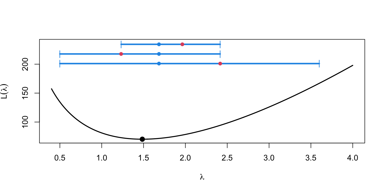
golden <- function(f, a, b, tol = 1e-8) {
  phi <- (sqrt(5) - 1) / 2; k <- 0
  x1 <- b - phi * (b - a); x2 <- a + phi * (b - a); f1 <- f(x1); f2 <- f(x2)
  while (b - a > tol) {
    if (f1 < f2) { b <- x2; x2 <- x1; f2 <- f1; x1 <- b - phi * (b - a); f1 <- f(x1) }
    else         { a <- x1; x1 <- x2; f1 <- f2; x2 <- a + phi * (b - a); f2 <- f(x2) }
    k <- k + 1 }
  c(root = (a + b) / 2, iter = k)
}
golden(nll, 0.1, 10)                     # R equivalent: optimize(nll, c(0.1, 10))

     root      iter 
 1.485204 44.000000 

Golden Section, Visualized

fv <- nll(lam); yr <- range(fv); pad <- 0.3 * diff(yr)
plot(lam, fv, type = "l", lwd = 2, ylim = c(yr[1], yr[2] + pad),
     xlab = TeX("$\\lambda$"), ylab = TeX("$L(\\lambda)$"))
points(lhat, nll(lhat), pch = 19, cex = 1.3)

gr <- (3 - sqrt(5)) / 2; xl <- 0.5; xu <- 3.6
ylev <- seq(yr[2] + 0.08 * pad, yr[2] + 0.95 * pad, length.out = 3)
for (k in 1:3) {
  xml <- xl + gr * (xu - xl); xmu <- xu - gr * (xu - xl)
  segments(xl, ylev[k], xu, ylev[k], col = 4, lwd = 3)
  points(c(xl, xu), rep(ylev[k], 2), pch = "|", col = 4)
  keep_lower <- nll(xml) < nll(xmu)
  points(xml, ylev[k], pch = 19, cex = 0.9, col = if (keep_lower) 4 else 2)
  points(xmu, ylev[k], pch = 19, cex = 0.9, col = if (keep_lower) 2 else 4)
  if (keep_lower) xu <- xmu else xl <- xml
}

The point that survives (blue) is already correctly placed for the next iteration, so only the red point costs a fresh evaluation.

Newton–Raphson: Derivation

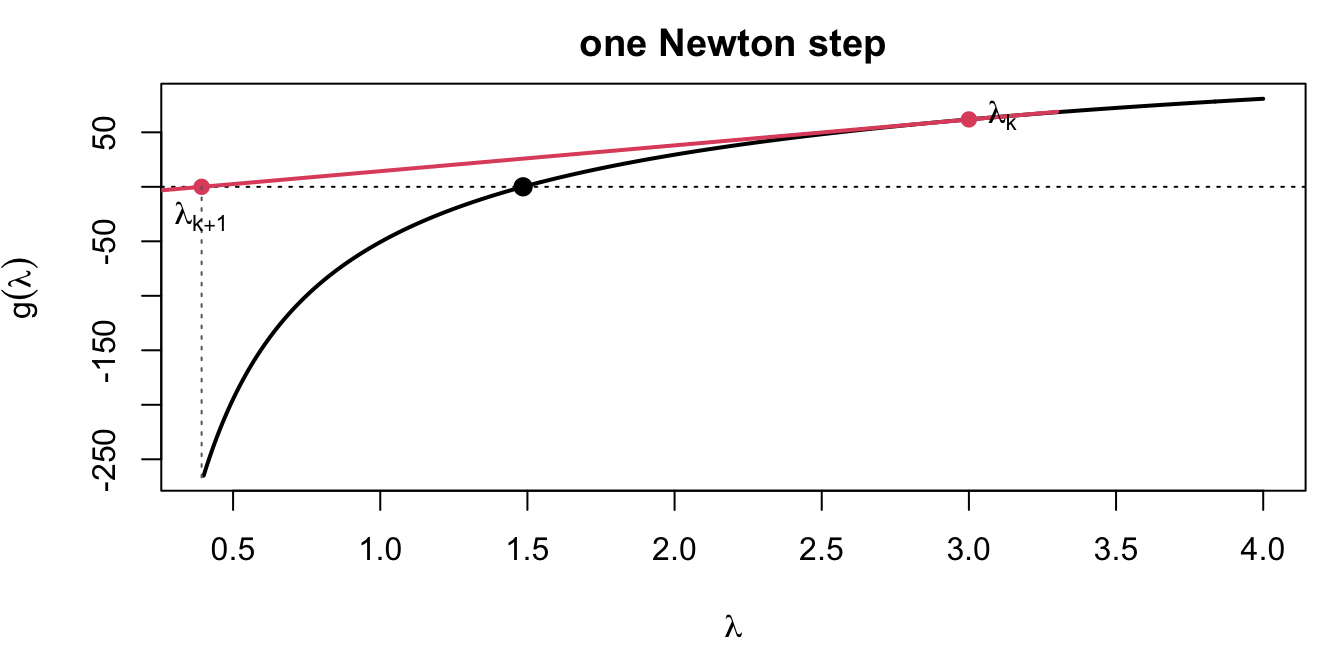
Approximate the gradient by its tangent line at the current point \theta_k and solve for where the tangent hits zero: g(\theta) \approx g(\theta_k) + g'(\theta_k)(\theta - \theta_k) = 0 \quad\Longrightarrow\quad \theta_{k+1} = \theta_k - \frac{g(\theta_k)}{g'(\theta_k)} = \theta_k - \frac{\mathcal{L}'(\theta_k)}{\mathcal{L}''(\theta_k)} .

Newton–Raphson: The Tangent Steps

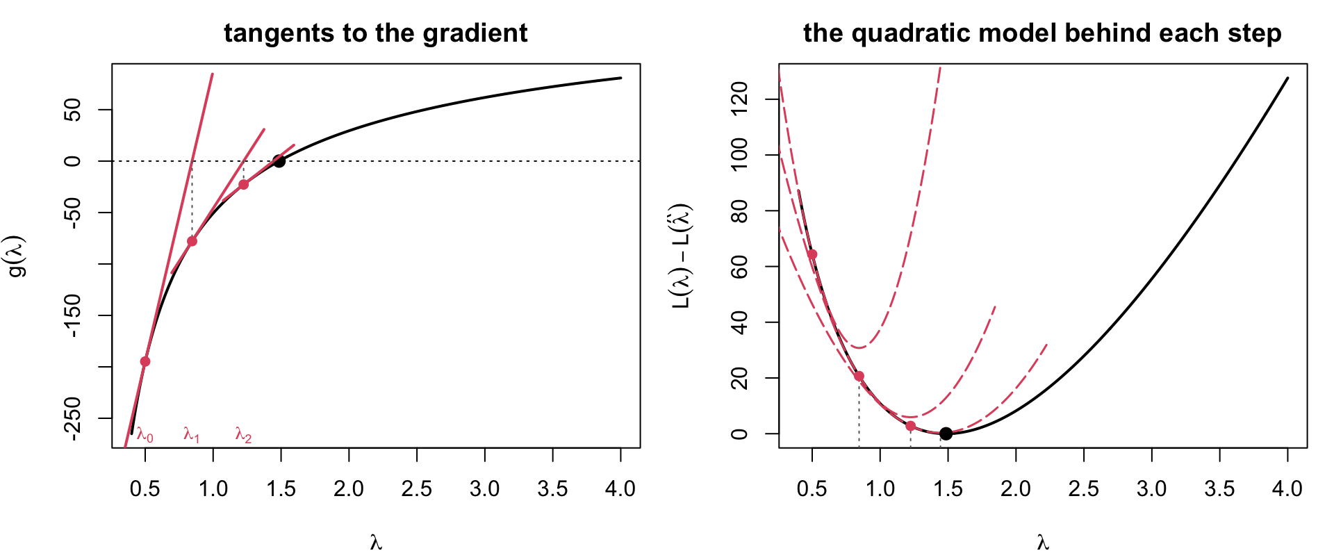
it <- 0.5                                        # starting value
for (k in 1:3) it <- c(it, it[k] - g(it[k]) / dg(it[k]))
par(mfrow = c(1, 2), mar = c(4.2, 4.2, 2.4, 1))

## (a) tangents to the gradient
plot(lam, g(lam), type = "l", lwd = 2, main = "tangents to the gradient",
     xlab = TeX("$\\lambda$"), ylab = TeX("$g(\\lambda)$"))
abline(h = 0, lty = 3); points(lhat, 0, pch = 19, cex = 1.2)
for (k in 1:3) {
  xt <- range(c(it[k], it[k + 1])) + c(-0.15, 0.15)
  lines(xt, g(it[k]) + dg(it[k]) * (xt - it[k]), col = 2, lwd = 2)
  segments(it[k + 1], 0, it[k + 1], g(it[k + 1]), lty = 3, col = "grey40")
  points(it[k], g(it[k]), pch = 19, col = 2, cex = 0.9)
  mtext(TeX(sprintf("$\\lambda_%d$", k - 1)), side = 1, at = it[k], line = -1, col = 2, cex = 0.8)
}

## (b) the quadratic model that each step minimizes
nllc <- function(l) nll(l) - nll(lhat)
plot(lam, nllc(lam), type = "l", lwd = 2, main = "the quadratic model behind each step",
     xlab = TeX("$\\lambda$"), ylab = TeX("$L(\\lambda) - L(\\hat{\\lambda})$"))
for (k in 1:3) {
  w <- seq(it[k] - 1, it[k] + 1, length.out = 200)
  lines(w, nllc(it[k]) + g(it[k]) * (w - it[k]) + 0.5 * dg(it[k]) * (w - it[k])^2,
        col = 2, lwd = 1.5, lty = 5)
  segments(it[k + 1], par("usr")[3], it[k + 1], nllc(it[k + 1]), lty = 3, col = "grey40")
  points(it[k], nllc(it[k]), pch = 19, col = 2, cex = 0.9)
}
points(lhat, 0, pch = 19, cex = 1.2)

Left: each red line is the tangent to g at the current iterate, followed down to the axis to give the next one. Right: the same steps seen on \mathcal{L} — the dashed parabola is the second-order Taylor expansion at \lambda_k, and \lambda_{k+1} is its vertex. As the iterates approach \hat\lambda the parabola hugs \mathcal{L} and the vertex lands essentially on the MLE.

Newton–Raphson in R

newton <- function(g, dg, x0, tol = 1e-8, maxit = 100, trace = FALSE) {
  for (k in 1:maxit) {
    x1 <- x0 - g(x0) / dg(x0)
    if (trace) cat(sprintf("iter %2d: %.10f\n", k, x1))
    if (!is.finite(x1)) stop("diverged")
    if (abs(x1 - x0) < tol) return(c(root = x1, iter = k))
    x0 <- x1 }
  stop("not converged")
}
newton(g, dg, x0 = xbar, trace = TRUE)

iter  1: 1.3823529274
iter  2: 1.4789563015
iter  3: 1.4851816577
iter  4: 1.4852043771
iter  5: 1.4852043774

    root     iter 
1.485204 5.000000 

Iteration counts on the same problem: fixed point 22, bisection 30, golden 40, Newton 5.

Convergence Rate of Newton–Raphson

Let e_k = \theta_k - \hat\theta. Expanding g(\hat\theta) = 0 around \theta_k: 0 = g(\theta_k) - g'(\theta_k)e_k + \tfrac12 g''(\xi)e_k^2 \quad\Longrightarrow\quad e_{k+1} = e_k - \frac{g(\theta_k)}{g'(\theta_k)} = \frac{g''(\xi)}{2g'(\theta_k)}\,e_k^2 .

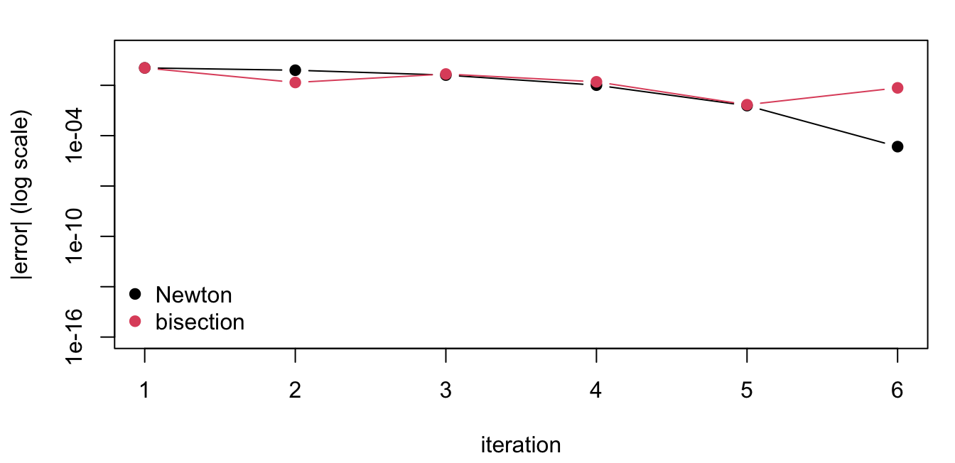
Quadratic convergence: the error is squared each step, so the number of correct digits roughly doubles. Linear methods gain a fixed number of digits per step.

When Newton–Raphson Fails

Newton uses only local information, so it can misbehave:

• Wrong curvature: if g'(\theta_k) = \mathcal{L}''(\theta_k) < 0, the step moves toward a maximum of \mathcal{L} or diverges.
• Overshooting: a flat gradient (g'(\theta_k) \approx 0) gives a huge step.
• Multiple roots: it converges to whichever root is nearest the start, possibly a local maximum.

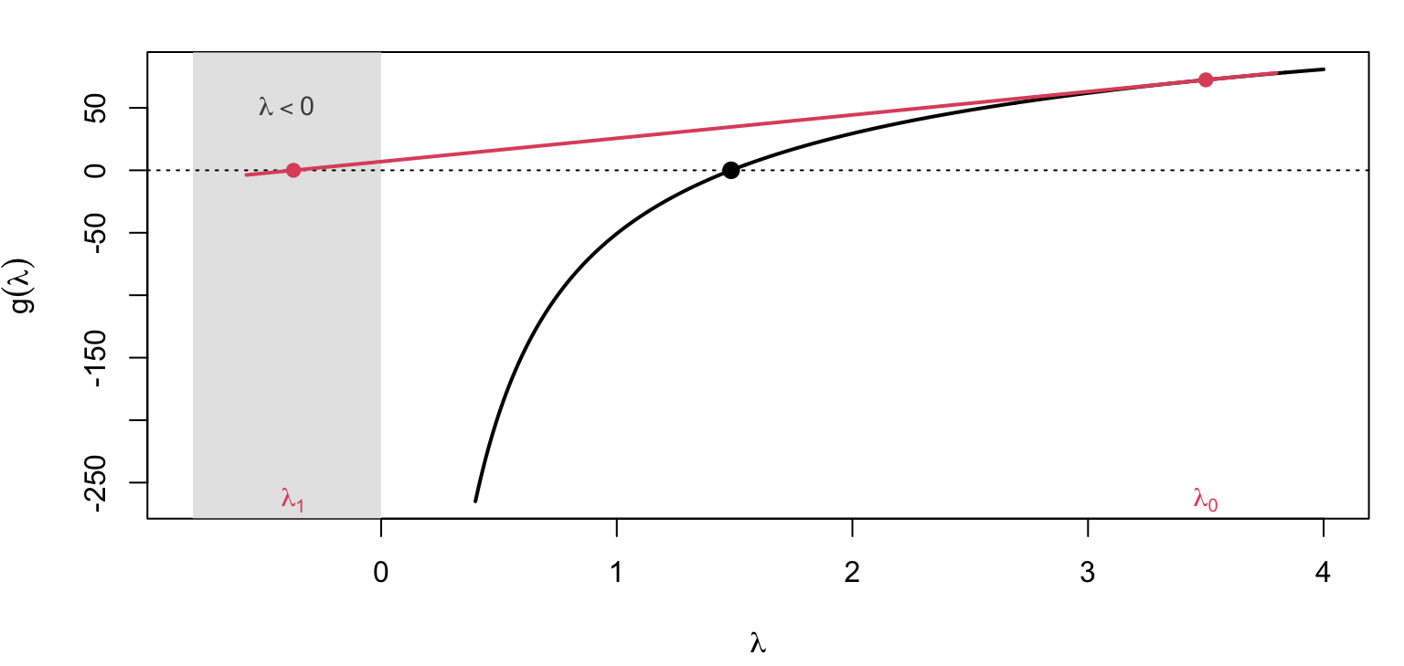
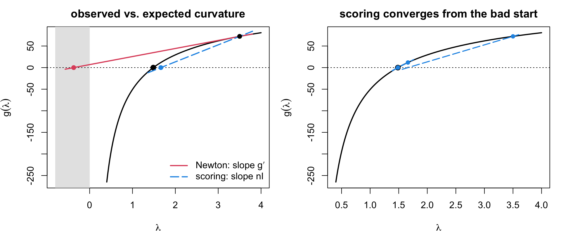
The truncated Poisson overshoots from a poor start: at \lambda_0 = 3.5 the gradient is already flat, so the tangent crosses zero outside the parameter space.

l0 <- 3.5; l_nr <- l0 - g(l0) / dg(l0)
par(mar = c(4.2, 4.2, 1.5, 1))
plot(NA, xlim = c(-0.8, 4), ylim = range(g(lam)),
     xlab = TeX("$\\lambda$"), ylab = TeX("$g(\\lambda)$"))
rect(-0.8, par("usr")[3], 0, par("usr")[4], col = "grey90", border = NA)
text(-0.4, 0.55 * par("usr")[4], TeX("$\\lambda < 0$"), col = "grey30", cex = 0.9)
lines(lam, g(lam), lwd = 2); abline(h = 0, lty = 3); points(lhat, 0, pch = 19, cex = 1.2)
xt <- c(l_nr - 0.2, l0 + 0.3)
lines(xt, g(l0) + dg(l0) * (xt - l0), col = 2, lwd = 2)
points(c(l0, l_nr), c(g(l0), 0), pch = 19, col = 2)
mtext(TeX("$\\lambda_0$"), side = 1, at = l0, line = -1, col = 2, cex = 0.9)
mtext(TeX("$\\lambda_1$"), side = 1, at = l_nr, line = -1, col = 2, cex = 0.9)

c(lambda_1 = l_nr)

  lambda_1 
-0.3720692 

tryCatch(newton(g, dg, l0), error = function(e) conditionMessage(e))

[1] "diverged"

Safeguards: start from a robust estimate, halve the step until \mathcal{L} decreases, or fall back to bisection/golden section, which only need a bracket.

Flat Tails: The Cauchy Location Model

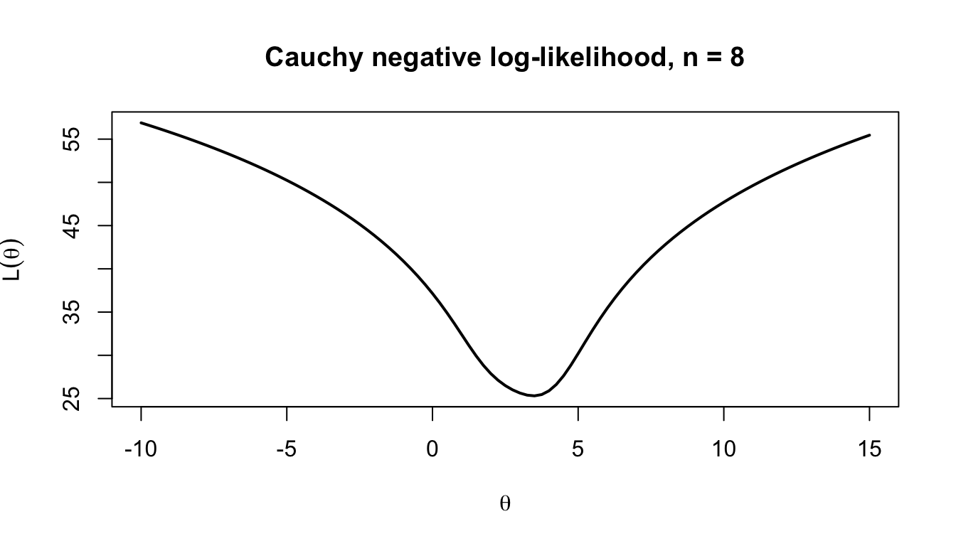
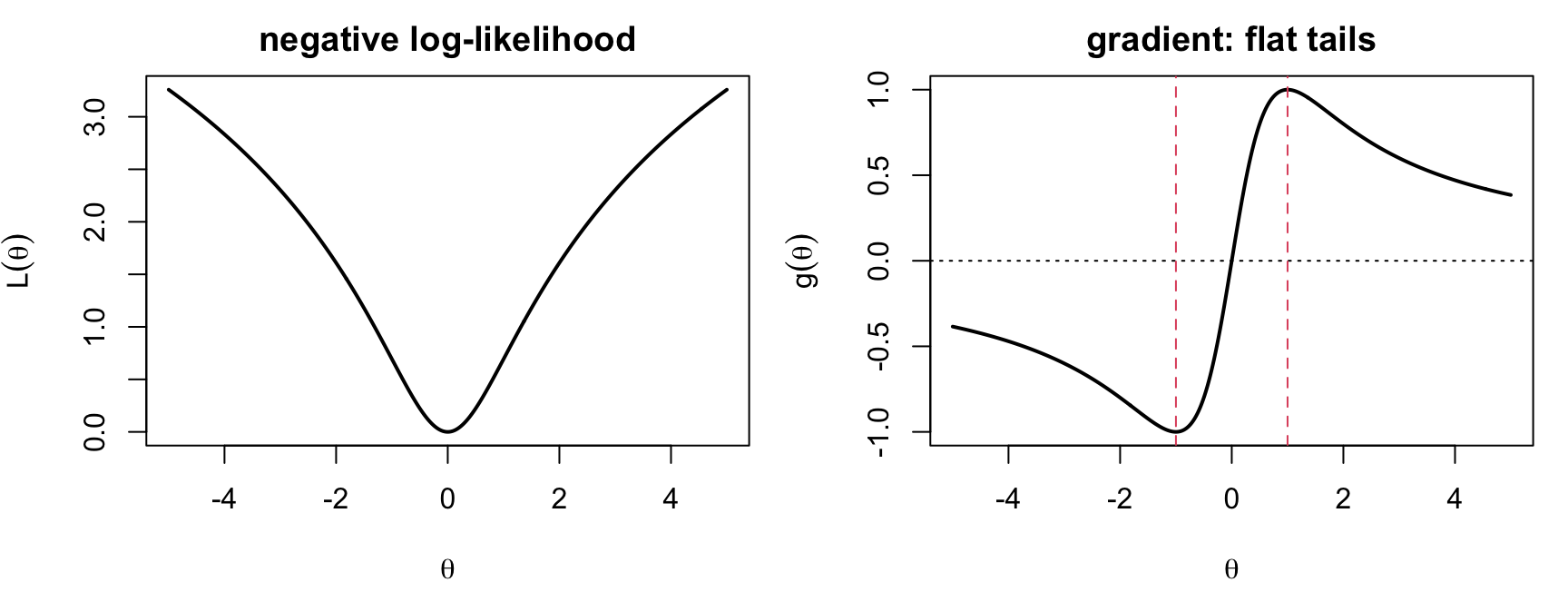
A single-observation Cauchy likelihood shows the same failure in pure form: \mathcal{L}(\theta) = -\ell(\theta) = \log(1+\theta^2) has gradient g(\theta) = 2\theta/(1+\theta^2), which rises, turns over at \theta = 1, then decays — the Newton step blows up wherever g is flat.

nll_c <- function(t) log(1 + t^2)
g_c   <- function(t) 2 * t / (1 + t^2)
par(mfrow = c(1, 2), mar = c(4.2, 4.2, 2.2, 1))
curve(nll_c, -5, 5, n = 400, lwd = 2, xlab = TeX("$\\theta$"), ylab = TeX("$L(\\theta)$"), main = "negative log-likelihood")
curve(g_c, -5, 5, n = 400, lwd = 2, xlab = TeX("$\\theta$"), ylab = TeX("$g(\\theta)$"), main = "gradient: flat tails")
abline(h = 0, lty = 3); abline(v = c(-1, 1), col = 2, lty = 2)

From \theta_0 = 0.5 Newton converges quadratically; from \theta_0 = 1.2, beyond the inflection point, it runs away — each step landing where the gradient is flatter still.

set.seed(2024)
x_c <- rcauchy(8, 3)
g_cau  <- function(t) sum(2 * (t - x_c) / (1 + (x_c - t)^2))       # gradient of the Cauchy nll
dg_cau <- function(t) sum(2 * (1 - (x_c - t)^2) / (1 + (x_c - t)^2)^2)
starts <- c(-5, 0, median(x_c), 8)
sapply(starts, function(s) tryCatch(newton(g_cau, dg_cau, s)["root"], error = function(e) NA))

[1] NA NA NA NA

Univariate Fisher Scoring

Replace the observed curvature J(\theta_k) = g'(\theta_k) by its expectation nI(\theta_k): \theta_{k+1} = \theta_k - \frac{g(\theta_k)}{n I(\theta_k)} .

• nI(\theta) > 0 always, so the step is always in a descent direction for \mathcal{L} — more robust than Newton far from the optimum.
• Near the MLE nI(\hat\theta) \approx g'(\hat\theta), so the two methods behave alike.
• Requires the expectation in closed form.

fisher_scoring <- function(g, nI, x0, tol = 1e-8, maxit = 100) {
  for (k in 1:maxit) { x1 <- x0 - g(x0) / nI(x0); if (abs(x1 - x0) < tol) return(c(root = x1, iter = k)); x0 <- x1 }
  stop("not converged")
}
rbind(newton = newton(g, dg, 3), scoring = fisher_scoring(g, nI, 3))

            root iter
newton  1.485204    8
scoring 1.485204    5

Newton vs. Scoring from the Same Point

par(mfrow = c(1, 2), mar = c(4.2, 4.2, 2.4, 1))

## (a) the two lines from the bad start
l_fs <- l0 - g(l0) / nI(l0)
plot(NA, xlim = c(-0.8, 4), ylim = range(g(lam)), main = "observed vs. expected curvature",
     xlab = TeX("$\\lambda$"), ylab = TeX("$g(\\lambda)$"))
rect(-0.8, par("usr")[3], 0, par("usr")[4], col = "grey90", border = NA)
lines(lam, g(lam), lwd = 2); abline(h = 0, lty = 3); points(lhat, 0, pch = 19, cex = 1.2)
xn <- c(l_nr - 0.2, l0 + 0.3); xf <- c(l_fs - 0.3, l0 + 0.3)
lines(xn, g(l0) + dg(l0) * (xn - l0), col = 2, lwd = 2)
lines(xf, g(l0) + nI(l0) * (xf - l0), col = 4, lwd = 2, lty = 5)
points(c(l0, l_nr, l_fs), c(g(l0), 0, 0), pch = 19, col = c(1, 2, 4))
legend("bottomright", bty = "n", lwd = 2, lty = c(1, 5), col = c(2, 4),
       legend = c(TeX("Newton: slope $g'$"), TeX("scoring: slope $nI$")))

## (b) the scoring path from the same start
plot(lam, g(lam), type = "l", lwd = 2, main = "scoring converges from the bad start",
     xlab = TeX("$\\lambda$"), ylab = TeX("$g(\\lambda)$"))
abline(h = 0, lty = 3); points(lhat, 0, pch = 19, cex = 1.2)
fs <- l0
for (k in 1:4) fs <- c(fs, fs[k] - g(fs[k]) / nI(fs[k]))
for (k in 1:4) {
  xt <- range(c(fs[k], fs[k + 1])) + c(-0.1, 0.1)
  lines(xt, g(fs[k]) + nI(fs[k]) * (xt - fs[k]), col = 4, lwd = 1.8, lty = 5)
  segments(fs[k + 1], 0, fs[k + 1], g(fs[k + 1]), lty = 3, col = "grey40")
  points(fs[k], g(fs[k]), pch = 19, col = 4, cex = 0.9)
}

c(newton_step = l_nr, scoring_step = l_fs)

 newton_step scoring_step 
  -0.3720692    1.6616773 

The two lines pass through the same point with different slopes. Newton uses the actual slope g'(\lambda_0), which is nearly flat here and throws the iterate out of the parameter space; scoring uses nI(\lambda_0), an average over hypothetical data, which stays steeply positive and keeps every iterate positive. The slopes agree as \lambda_k \to \hat\lambda, so the two methods finish at the same speed.

Standard Error from the Curvature

At the MLE \hat\lambda, the observed information J(\hat\lambda) = \mathcal{L}''(\hat\lambda) = g'(\hat\lambda) and the expected information nI(\hat\lambda) both estimate the precision:

c(mle = lhat, se_observed = 1 / sqrt(dg(lhat)), se_expected = 1 / sqrt(nI(lhat)))

        mle se_observed se_expected 
  1.4852044   0.1164092   0.1164092 

lhat + c(-1.96, 1.96) / sqrt(dg(lhat))    # 95% Wald interval

[1] 1.257042 1.713366

Numerical Derivatives

When g or g' is tedious to derive, approximate by finite differences: g(\theta) = \mathcal{L}'(\theta) \approx \frac{\mathcal{L}(\theta + h) - \mathcal{L}(\theta - h)}{2h}, g'(\theta) = \mathcal{L}''(\theta) \approx \frac{\mathcal{L}(\theta + h) - 2\mathcal{L}(\theta) + \mathcal{L}(\theta - h)}{h^2}.

• h too large: truncation error; h too small: roundoff error (large − large). Typical choice h \approx \sqrt{\epsilon}\,(1 + \lvert\theta\rvert) \approx 10^{-8} for the first derivative, \epsilon^{1/3} for the second.

• R’s nlm() and optim(method = "BFGS") use numerical gradients unless you supply analytic ones; numDeriv::grad() and hessian() are more accurate.

h <- 1e-5
c(analytic = dg(lhat), numeric = (nll(lhat + h) - 2 * nll(lhat) + nll(lhat - h)) / h^2)

analytic  numeric 
73.79477 73.79498 

Does the Effort Pay Off? MLE vs. the Naive Estimator

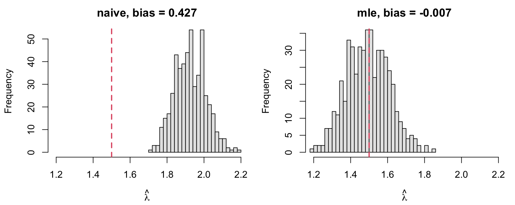
Simulating many truncated samples shows the naive estimator’s bias never vanishes — it is the wrong model, not too little data — while the MLE is centred on the truth.

mle_nzp <- function(n_obs)
  uniroot(function(l) length(n_obs) / (1 - exp(-l)) - sum(n_obs) / l,
          c(1e-6, 50), tol = 1e-10)$root

sim_nzp <- function(lambda, n_gen = 200, B = 500)
  vapply(1:B, function(b) {
    yb <- rpois(n_gen, lambda); nb <- yb[yb > 0]
    c(naive = mean(nb), mle = mle_nzp(nb))
  }, c(naive = 0, mle = 0))

est <- sim_nzp(1.5)
par(mfrow = c(1, 2), mar = c(4.2, 4.2, 2.2, 1))
for (m in c("naive", "mle"))
  { hist(est[m, ], breaks = 25, col = "grey90", xlim = range(est),
         xlab = TeX("$\\hat{\\lambda}$"),
         main = sprintf("%s, bias = %.3f", m, mean(est[m, ]) - 1.5))
    abline(v = 1.5, col = 2, lwd = 2, lty = 2) }

The naive estimator’s bias grows as \lambda shrinks, since more mass sits on the discarded zero; the MLE’s spread matches the information-based standard error from two slides ago.

3 Multivariate Newton–Raphson and Fisher Scoring

Gradient and Hessian

For \theta = (\theta_1, \ldots, \theta_p)', the gradient and Hessian of \mathcal{L} are g(\theta) = \nabla\mathcal{L}(\theta) = \begin{pmatrix}\partial\mathcal{L}/\partial\theta_1 \\ \vdots \\ \partial\mathcal{L}/\partial\theta_p\end{pmatrix}, \qquad H(\theta) = \nabla^2\mathcal{L}(\theta) = \left(\frac{\partial^2\mathcal{L}}{\partial\theta_i\,\partial\theta_j}\right)_{p\times p} .

• g points in the direction of steepest ascent of \mathcal{L} and is perpendicular to the contour through \theta; every method below moves along -g.

• H describes the local curvature. At a local minimum it is positive semidefinite; if it is positive definite, the minimum is strict and locally unique. Near the minimum, \mathcal{L} is well approximated by a quadratic, so H determines the shape of the contours. At the MLE, H(\hat\theta) = J(\hat\theta), the observed information.

Gradient and Hessian: Illustration

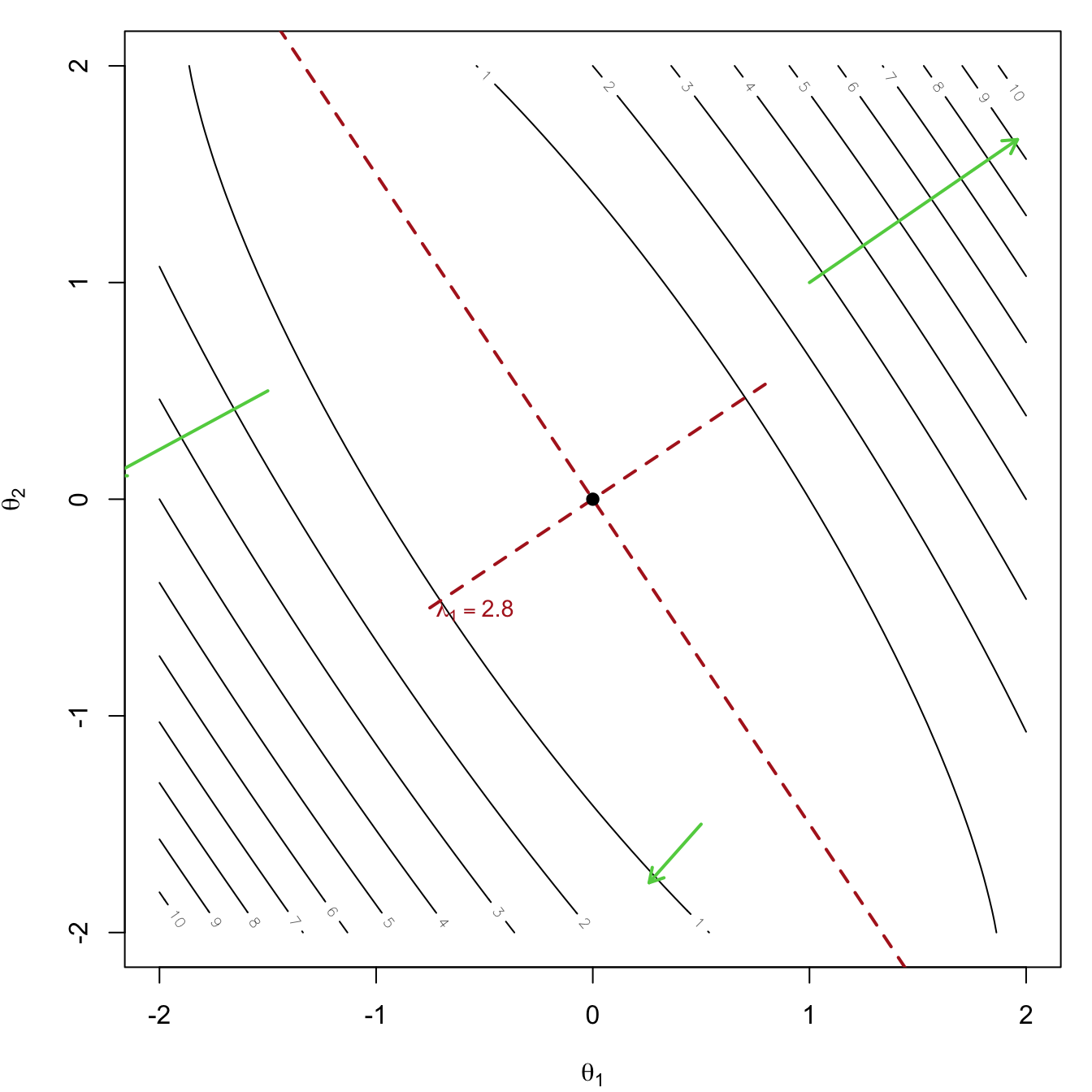
Quadratic: \mathcal{L}(\theta) = \tfrac12(\theta - u)'A(\theta - u), A positive definite, g(\theta) = A(\theta - u), H = A (constant). Contours are ellipses centred at u. Write A = Q\Lambda Q':

• axes point along the eigenvectors of Q;
• half-length along axis j is \propto 1/\sqrt{\lambda_j}, so a large eigenvalue means high curvature and a short, well-determined direction;
• \lambda_{\max}/\lambda_{\min} measures elongation; tilted ellipses indicate correlated parameters.
• Gradient arrows (green) are perpendicular to contours and point uphill, away from u; a descent method steps along -g, which need not point at u unless the ellipse is a circle.
• Near its minimum any smooth \mathcal{L} looks like this, with A = \nabla^2\mathcal{L}(\hat\theta) = J(\hat\theta).

Multivariate Newton–Raphson

Second-order Taylor expansion at \theta_k, minimized exactly: \mathcal{L}(\theta) \approx \mathcal{L}(\theta_k) + g(\theta_k)'(\theta - \theta_k) + \tfrac12(\theta - \theta_k)'H(\theta_k)(\theta - \theta_k) \Longrightarrow\quad \underbrace{\theta_{k+1}}_{p\times1} = \theta_k - \underbrace{\big[H(\theta_k)\big]^{-1}}_{p\times p}\underbrace{g(\theta_k)}_{p\times1}.

Compare with the univariate \theta_{k+1} = \theta_k - g(\theta_k)/g'(\theta_k): division becomes multiplication by the inverse Hessian.

Fisher scoring replaces H(\theta_k) = \nabla^2\mathcal{L}(\theta_k) by the expected information nI(\theta_k): \theta_{k+1} = \theta_k - \big[nI(\theta_k)\big]^{-1}g(\theta_k).

Each iteration costs one p \times p linear solve — O(p^3) — fine for p in the hundreds, expensive for p in the millions.

Example: Logistic Regression

y_i \mid x_i \sim \mathrm{Bern}(\pi_i) with \pi_i = \dfrac{e^{\eta_i}}{1 + e^{\eta_i}} = \dfrac{1}{1 + e^{-\eta_i}}, \eta_i = x_i'\beta, x_i = (1, x_{i1}, \ldots, x_{ip})'. L(\beta) = \prod_{i=1}^n \pi_i^{y_i}(1-\pi_i)^{1-y_i} = \prod_{i=1}^n \frac{e^{y_i\eta_i}}{1 + e^{\eta_i}} \mathcal{L}(\beta) = \sum_{i=1}^n \big[\log(1 + e^{x_i'\beta}) - y_i\,x_i'\beta\big].

Using \dfrac{\partial}{\partial\beta}\log(1 + e^{x_i'\beta}) = \pi_i x_i and \dfrac{\partial\pi_i}{\partial\beta} = \pi_i(1-\pi_i)x_i: g(\beta) = \sum_{i=1}^n (\pi_i - y_i)\,x_i = X'(\pi - y), \qquad H(\beta) = \sum_{i=1}^n \pi_i(1-\pi_i)\,x_i x_i' = X'WX, \text{with}~W = \mathrm{diag}\big(\pi_i(1-\pi_i)\big) .

Logistic Regression: Newton = Fisher Scoring = IRLS

• H = X'WX is positive semi-definite, so \mathcal{L} is convex: any stationary point is the global minimum.

• The Hessian does not involve y, so its expectation equals itself: Newton–Raphson and Fisher scoring coincide.

• The update \beta_{k+1} = \beta_k - (X'W_kX)^{-1}X'(\pi_k - y) = (X'W_kX)^{-1}X'W_k z_k, z_k = X\beta_k + W_k^{-1}(y - \pi_k), is a weighted least squares fit of the working response z_k: iteratively reweighted least squares (IRLS), which is how glm() fits all generalized linear models.

• Caveat: if the classes are perfectly separable, \mathcal{L} decreases forever and the MLE does not exist (\lvert\hat\beta\rvert \to \infty).

Logistic Regression in R

n <- 500; X <- cbind(1, rnorm(n), rnorm(n)); beta_true <- c(-0.5, 1, -2)
y <- rbinom(n, 1, plogis(X %*% beta_true))
nll_lr <- function(b) sum(log1p(exp(X %*% b)) - y * (X %*% b))
g_lr   <- function(b) crossprod(X, plogis(X %*% b) - y)
H_lr   <- function(b) { p <- plogis(X %*% b); crossprod(X, X * drop(p * (1 - p))) }

newton_mv <- function(g, H, b0, tol = 1e-8, maxit = 50) {
  path <- drop(b0)
  for (k in 1:maxit) {
    b1 <- b0 - solve(H(b0), g(b0)); path <- rbind(path, drop(b1))
    if (max(abs(b1 - b0)) < tol)
      return(list(est = drop(b1), iter = k, se = sqrt(diag(solve(H(b1)))), path = path))
    b0 <- b1 }
}
fit <- newton_mv(g_lr, H_lr, rep(0, 3)); fit$iter

[1] 7

rbind(newton = fit$est, glm = coef(glm(y ~ X[, -1], family = binomial)))

       (Intercept)  X[, -1]1  X[, -1]2
newton  -0.5956291 0.8618954 -1.840956
glm     -0.5956291 0.8618954 -1.840956

rbind(newton = fit$se, glm = sqrt(diag(vcov(glm(y ~ X[, -1], family = binomial)))))

       (Intercept)  X[, -1]1  X[, -1]2
newton   0.1216455 0.1298958 0.1790956
glm      0.1216448 0.1298948 0.1790936

Variance of the MLE \hat\beta

\widehat{\mathrm{Var}}(\hat\beta) = \big[\nabla^2\mathcal{L}(\hat\beta)\big]^{-1} = J(\hat\beta)^{-1} = (X'\hat WX)^{-1} = \begin{pmatrix}\hat\sigma_{00} & \cdots & \hat\sigma_{0p} \\ \vdots & \ddots & \vdots \\ \hat\sigma_{p0} & \cdots & \hat\sigma_{pp}\end{pmatrix}, \widehat{\mathrm{SE}}(\hat\beta_j) = \sqrt{\hat\sigma_{jj}} .

Wald tests and confidence intervals follow directly: z_j = \frac{\hat\beta_j}{\widehat{\mathrm{SE}}(\hat\beta_j)} \;\dot\sim\; N(0,1) \text{ under } H_0: \beta_j = 0, \qquad \hat\beta_j \pm 1.96\,\widehat{\mathrm{SE}}(\hat\beta_j).

This is the summary(glm(...)) table. The variance comes from the same Hessian that drove the Newton iterations.

The Need to Robustify Newton–Raphson

The Newton step d_k = -H_k^{-1} g_k, with g_k = \nabla\mathcal{L}(\theta_k) and H_k = \nabla^2\mathcal{L}(\theta_k), solves the local quadratic model exactly. Two things can go wrong away from the solution:

• The direction may not descend. g_k^\top d_k = -g_k^\top H_k^{-1} g_k < 0 requires H_k \succ 0. Where \mathcal{L} is not convex, H_k may be indefinite or singular and d_k can point uphill.
• The unit step may overshoot. Even with H_k \succ 0, the quadratic model is trustworthy only near \theta_k; \alpha_k = 1 can increase \mathcal{L}.

The two failures are independent and need separate remedies: one fixes the direction, the other the length.

Robustification of the Hessian

Replace H_k by a positive definite \tilde H_k and solve \tilde H_k d_k = -g_k.

Shift by a multiple of the identity. With \lambda_{\min} the smallest eigenvalue of H_k, \tilde H_k = H_k + \tau I, \qquad \tau = \max\left(0,\; \delta - \lambda_{\min}\right), \qquad \delta = 10^{-3}\lambda_{\max} . Eigenvectors are unchanged and every eigenvalue is shifted by \tau. As \tau \to \infty the direction rotates toward -g_k, so the method interpolates between Newton and steepest descent.

Spectral modification. With H_k = V \Lambda V^\top, replace \lambda_i by \max(|\lambda_i|, \delta). This reverses negative-curvature directions rather than damping them, so the step moves away from a saddle.

Where H_k \succ 0 already, \tau = 0 and \tilde H_k = H_k: the refinement is inactive near a well-behaved minimum.

Step length: backtracking and line search

Given a descent direction, choose \alpha_k by an inexact search along \phi(\alpha) = \mathcal{L}(\theta_k + \alpha d_k).

Armijo (sufficient decrease). \mathcal{L}(\theta_k + \alpha d_k) \le \mathcal{L}(\theta_k) + c_1 \alpha\, g_k^\top d_k, \qquad c_1 = 10^{-4}.

Backtracking. Start at \alpha = 1 and set \alpha \leftarrow \rho\alpha with \rho = \tfrac12 until Armijo holds. Simple, and it accepts \alpha_k = 1 whenever the full Newton step is acceptable.

Curvature (Wolfe) condition. g(\theta_k + \alpha d_k)^\top d_k \ \ge\ c_2\, g_k^\top d_k, \qquad c_2 = 0.9, which rules out steps that are too short. Backtracking alone cannot enforce it, since it never lengthens the trial step. The condition matters for conjugate gradient and is what keeps s_k^\top y_k > 0, hence the BFGS update well defined.

The safeguarded algorithm

At \theta_k: compute g_k, H_k; form \tilde H_k \succ 0; solve \tilde H_k d_k = -g_k; find \alpha_k from \alpha_0 = 1 by line search; set \theta_{k+1} = \theta_k + \alpha_k d_k.

Both safeguards are needed, and both switch themselves off:

	near a minimum	far away / indefinite
\tau	0	> 0, direction rotates toward -g_k
\alpha_k	1	< 1 (or > 1 under Wolfe)

Quadratic convergence is therefore retained locally, while sufficient decrease at every iteration gives convergence from remote starting points. This is safeguarded Newton, not “Newton–Raphson” in the textbook sense — and not what nlm() runs, which globalizes with a trust region.

4 Gradient-based Methods

What If the Hessian Is Unavailable or Too Big?

method	uses	per-iteration cost	typical use
Nelder–Mead	\mathcal{L} only	O(p) evaluations	small p, non-smooth or noisy \mathcal{L}
gradient descent + line search	g	O(p) + line search	large p
conjugate gradient	g	O(p) + line search	large p, quadratic-like \mathcal{L}
quasi-Newton (BFGS, L-BFGS)	g, builds \approx Hessian	O(p^2) / O(mp)	default general-purpose
Newton / Fisher scoring	g, H	O(p^3)	moderate p, gives SEs

All are available through optim(par, fn, gr, method = ...) in R. Convention below: minimize \mathcal{L}(\theta) = -\ell(\theta), with g = \nabla\mathcal{L}.

Gradient Descent with Line Search

Move in the direction of steepest descent d_k = -g(\theta_k), choosing the step length \alpha_k by a line search: \theta_{k+1} = \theta_k + \alpha_k d_k, \qquad \alpha_k = \arg\min_{\alpha > 0} \mathcal{L}(\theta_k + \alpha d_k) .

• Exact line search: a univariate minimization (golden section / optimize) along the ray.

• Inexact (backtracking, Armijo): start with \alpha = 1 and halve until \mathcal{L}(\theta_k + \alpha d_k) \le \mathcal{L}(\theta_k) + c\,\alpha\,g(\theta_k)'d_k (a “sufficient decrease”).

grad_descent <- function(nll, g, x0, maxit = 1000, tol = 1e-8) {
  path <- x0
  for (k in 1:maxit) {
    d <- -g(x0); a <- optimize(function(a) nll(x0 + a * d), c(0, 10))$minimum   # exact line search
    x1 <- x0 + a * d; path <- rbind(path, x1)
    if (sqrt(sum((x1 - x0)^2)) < tol) break
    x0 <- x1 }
  list(par = x1, iter = k, path = path)
}

Why Gradient Descent Zig-Zags

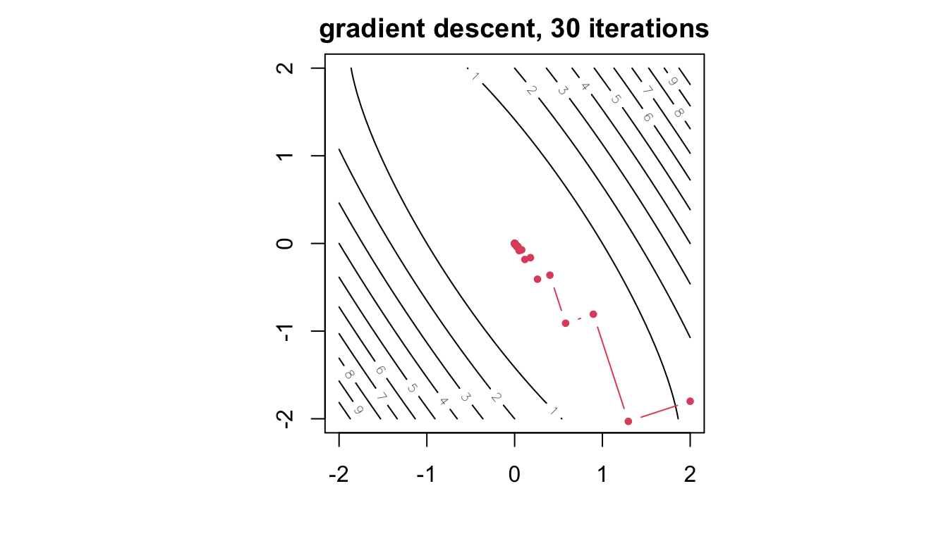
With exact line search, consecutive directions are orthogonal (g(\theta_{k+1})'d_k = 0), so on elongated contours the path zig-zags across the valley:

The number of iterations grows with the condition number of the Hessian (ratio of largest to smallest eigenvalue).

Conjugate Gradient

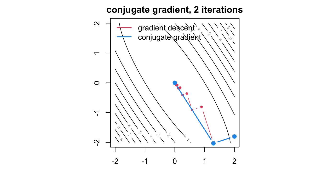
Fix the zig-zag by making each new direction conjugate to the previous ones with respect to the Hessian Q: d_i'Qd_j = 0 for i \ne j. For a quadratic \mathcal{L}(\theta) = \tfrac12\theta'Q\theta - b'\theta, minimizing along p such directions reaches the exact minimum in at most p steps.

The nonlinear version builds directions from gradients only: d_0 = -g_0, \qquad d_{k+1} = -g_{k+1} + \beta_k d_k, \qquad \beta_k^{FR} = \frac{g_{k+1}'g_{k+1}}{g_k'g_k}\ \text{(Fletcher–Reeves)}, \quad \beta_k^{PR} = \frac{g_{k+1}'(g_{k+1} - g_k)}{g_k'g_k}\ \text{(Polak–Ribière)}, with \theta_{k+1} = \theta_k + \alpha_k d_k from a line search and g_k = g(\theta_k) = \nabla\mathcal{L}(\theta_k).

• Memory: only two vectors. No matrix ever formed. Ideal for very large p.

• Restart with d = -g_k every p iterations, since conjugacy degrades on non-quadratic \mathcal{L}.

Conjugate Gradient in R

conj_grad <- function(nll, g, x0, maxit = 1000, tol = 1e-8, restart = length(x0)) {
  g0 <- g(x0); d <- -g0; path <- x0
  for (k in 1:maxit) {
    a <- optimize(function(a) nll(x0 + a * d), c(0, 10))$minimum
    x1 <- x0 + a * d; g1 <- g(x1); path <- rbind(path, x1)
    if (sqrt(sum(g1^2)) < tol) break
    beta <- if (k %% restart == 0) 0 else max(0, sum(g1 * (g1 - g0)) / sum(g0^2))   # Polak-Ribiere+
    d <- -g1 + beta * d; x0 <- x1; g0 <- g1 }
  list(par = x1, iter = k, path = path)
}
cg <- conj_grad(nllq, gq, c(2, -1.8))
par(pty = "s", mar = c(4, 4, 2, 1)); contour(seq(-2, 2, l = 80), seq(-2, 2, l = 80), z, nlevels = 15, main = sprintf("conjugate gradient, %d iterations", cg$iter))
lines(gd$path, type = "b", col = 2, pch = 19, cex = 0.6); lines(cg$path, type = "b", col = 4, pch = 19, lwd = 2)
legend("topleft", c("gradient descent", "conjugate gradient"), col = c(2, 4), lwd = 2, bty = "n")

Quasi-Newton: BFGS

Between gradient methods and Newton: build an approximation B_k \approx \nabla^2\mathcal{L} from successive gradient differences s_k = \theta_{k+1} - \theta_k, y_k = g_{k+1} - g_k, via a rank-two update that keeps B_k positive definite. Steps are d_k = -B_k^{-1}g_k with a line search.

g_lr_vec <- function(b) drop(g_lr(b))
fits <- list(NM = optim(rep(0, 3), nll_lr, method = "Nelder-Mead"),
             CG = optim(rep(0, 3), nll_lr, g_lr_vec, method = "CG"),
             BFGS = optim(rep(0, 3), nll_lr, g_lr_vec, method = "BFGS", hessian = TRUE))
t(sapply(fits, function(f) c(f$par, f_evals = f$counts[1], g_evals = f$counts[2])))

                                    f_evals.function g_evals.gradient
NM   -0.5958732 0.8617178 -1.841346               98               NA
CG   -0.5956291 0.8618954 -1.840956               73               25
BFGS -0.5956291 0.8618954 -1.840956               35               13

sqrt(diag(solve(fits$BFGS$hessian)))     # SEs from the numerically computed Hessian at the optimum

[1] 0.1216455 0.1298958 0.1790956

optim(..., hessian = TRUE) returns a finite-difference Hessian at the solution, so standard errors are available even for gradient-only methods.

5 Stochastic Gradient Descent

Motivation: Large n

For iid data the negative log-likelihood and its gradient are sums over observations: \mathcal{L}(\theta) = \sum_{i=1}^n \mathcal{L}_i(\theta), \qquad g(\theta) = \sum_{i=1}^n g_i(\theta), \qquad g_i = \nabla\mathcal{L}_i .

Every method so far needs the full gradient, an O(np) pass through all data, per iteration (and Newton needs O(np^2) for the Hessian). With n in the millions and p in the millions (neural networks), even one full gradient is expensive.

Idea. g_i(\theta) for a randomly chosen i is an unbiased estimate of the average gradient: E_i\big[g_i(\theta)\big] = \frac{1}{n}\,g(\theta).

A noisy but cheap gradient estimate is enough to make progress — a Monte Carlo idea applied to optimization.

The SGD Algorithm

For t = 1, 2, \ldots:

1. Sample an index i_t uniformly from \{1, \ldots, n\} (or shuffle the data and cycle through it; one pass is an epoch).

2. Update in the descent direction of that single observation’s negative log-likelihood: \theta_{t+1} = \theta_t - \gamma_t\,g_{i_t}(\theta_t).

Mini-batch SGD averages the gradient over a batch B_t of m observations (m = 32–512 typical): \theta_{t+1} = \theta_t - \gamma_t\,\frac{1}{m}\sum_{i\in B_t}g_i(\theta_t), reducing the variance by 1/m at m times the cost, and using vectorized/GPU arithmetic.

The learning rate \gamma_t replaces the line search (a line search would need full-data evaluations).

Learning Rate and Convergence

Because the gradient is noisy, a constant \gamma makes \theta_t bounce around the optimum with variance \propto \gamma. Robbins–Monro (1951): convergence to the optimum is guaranteed if \sum_t \gamma_t = \infty \quad\text{and}\quad \sum_t \gamma_t^2 < \infty, \qquad\text{e.g. } \gamma_t = \frac{\gamma_0}{1 + t/t_0} .

• \gamma too large: divergence or persistent noise. \gamma too small: painfully slow.

• Convergence is only sublinear, far slower than Newton per iteration — but each iteration costs O(p) instead of O(np), and early progress is fast.

• Common refinements: momentum (average past gradients), Adam (per-coordinate adaptive rates), averaging the iterates \overline\theta_T = \frac1T\sum_t\theta_t (Polyak–Ruppert), which restores the \sqrt n-efficiency of the MLE.

A Smaller Logistic Regression, for SGD

Let’s apply SGD to logistic regrression.

log1pexp <- function(u) pmax(u, 0) + log1p(exp(-abs(u)))
nll_g_info <- function(b, r, z) {
  u <- b[1] + b[2] * z; p <- plogis(u); w <- p * (1 - p)
  list(nll  = -sum(u * r - log1pexp(u)),                   # L(beta)
       g    = c(sum(p - r), sum(z * (p - r))),             # g(beta) = grad L
       info = matrix(c(sum(w), sum(z * w), sum(z * w), sum(z * z * w)), 2, 2))
}
nll_logistic <- function(b, z, r) { u <- b[1] + b[2] * z; -sum(u * r - log1pexp(u)) }
mle_logistic_nr <- function(b0, no_iter, r, z) {
  out <- matrix(NA_real_, no_iter + 1, 3, dimnames = list(NULL, c("beta0", "beta1", "nll")))
  b <- b0
  for (i in seq_len(no_iter + 1)) {
    q <- nll_g_info(b, r, z); out[i, ] <- c(b, q$nll)
    if (i > no_iter) break
    step <- tryCatch(solve(q$info, q$g), error = function(e) rep(NA_real_, 2))
    if (any(!is.finite(step))) break
    b <- b - step
  }
  out
}

set.seed(1)
n2 <- 200; z2 <- sort(runif(n2, -2, 2)); r2 <- rbinom(n2, 1, plogis(1.5 * z2))
logit_nlm <- nlm(nll_logistic, c(0, 0), z = z2, r = r2, hessian = TRUE)
logit_nlm$estimate

[1] -0.2725325  1.5034237

Example: SGD for Logistic Regression in R

sgd_logistic <- function(z, r, b0, gamma0 = 0.5, t0 = 100, epochs = 30, batch = 10) {
  n <- length(z); b <- b0; t <- 0; path <- b0
  for (e in 1:epochs) {
    idx <- sample(n)
    for (s in seq(1, n, by = batch)) {
      i <- idx[s:min(s + batch - 1, n)]
      t <- t + 1
      u <- b[1] + b[2] * z[i]
      p <- plogis(u)
      gb <- c(sum(p - r[i]), sum(z[i] * (p - r[i]))) / length(i)   # batch gradient of L
      b <- b - gamma0 / (1 + t / t0) * gb
      path <- rbind(path, b)
    }
  }
  list(est = b, path = path)
}

set.seed(2)
beta_true2 <- c(0, 1.5)
sg <- sgd_logistic(z2, r2, c(0, 0))
rbind(sgd = sg$est, nlm = logit_nlm$estimate, truth = beta_true2)

            [,1]     [,2]
sgd   -0.2665590 1.506754
nlm   -0.2725325 1.503424
truth  0.0000000 1.500000

SGD Trajectory vs. Newton–Raphson

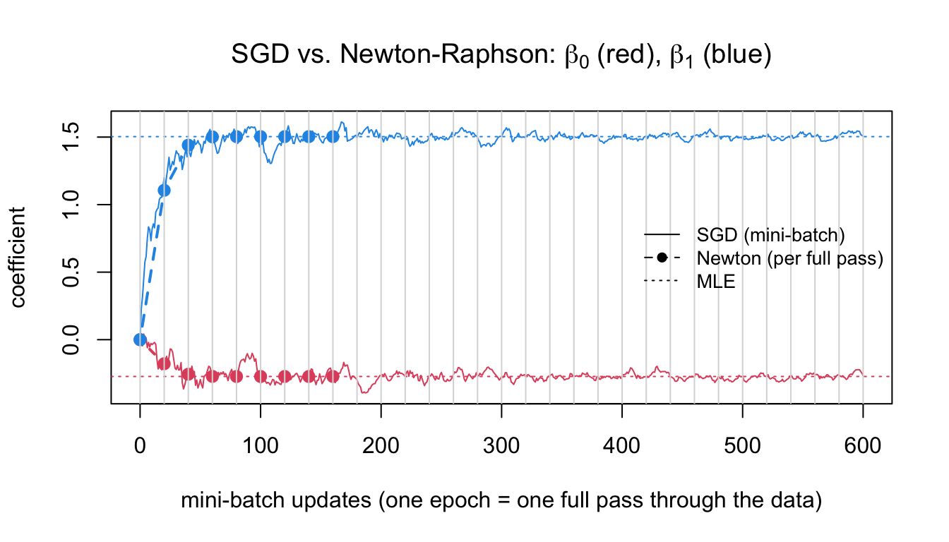
• Newton–Raphson needed 7 full-data passes; SGD made 600 cheap updates over 5 epochs and lands near the MLE with residual noise.

• Per data pass, Newton–Raphson is far more efficient here (n = 500, p = 3); SGD earns its keep when one full gradient — or the O(p^3) Hessian solve — is prohibitively expensive.

6 Nelder–Mead (Simplex Method)

Overview

Maintains a simplex of p+1 points (a triangle in 2D) and moves it downhill using only function values:

1. Order the vertices f(\theta_{(1)}) \le \cdots \le f(\theta_{(p+1)}); let \overline\theta be the centroid of the best p.

2. Reflect the worst vertex through \overline\theta; if the reflected point is the new best, try expanding further.

3. If reflection is poor, contract toward \overline\theta; if that also fails, shrink all vertices toward the best.

rosen <- function(v) (1 - v[1])^2 + 100 * (v[2] - v[1]^2)^2       # Rosenbrock "banana", min at (1, 1)
nm <- optim(c(-1.2, 1), rosen, method = "Nelder-Mead"); c(nm$par, evals = nm$counts["function"])

                              evals.function 
      1.000260       1.000506     195.000000 

Robust and derivative-free (R’s optim default), but slow in high dimensions and offers no standard errors.

Nelder–Mead: The Simplex Moves

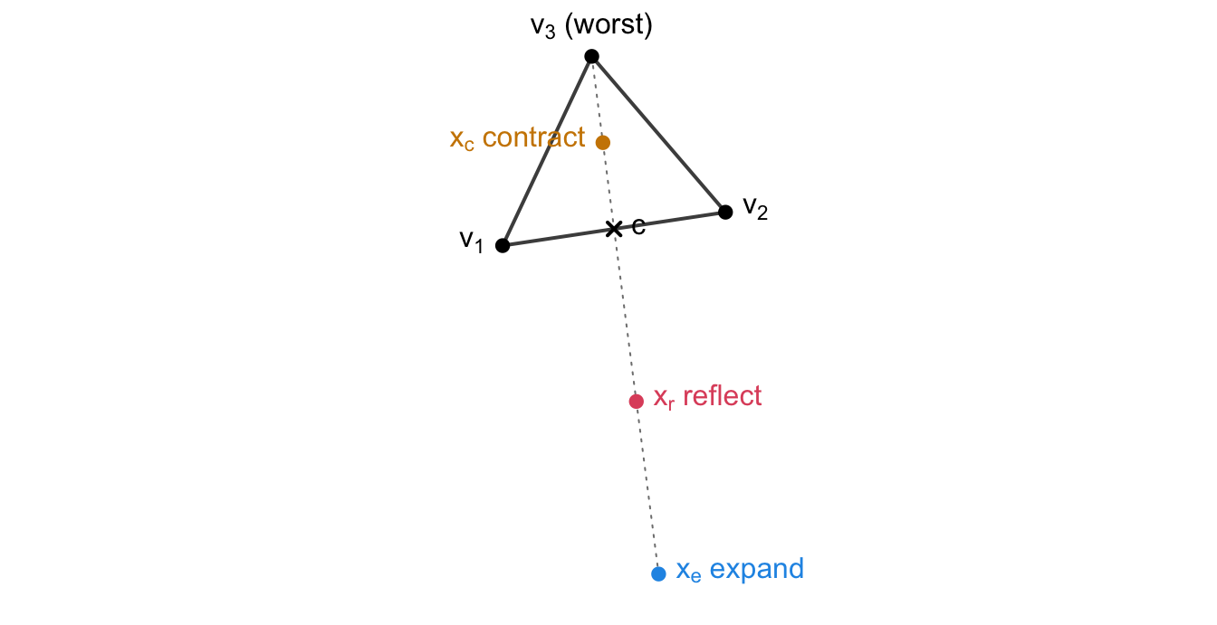
Golden section needs a bracket, which exists only in one dimension. Nelder–Mead generalizes the idea: keep d+1 points (a simplex) in \mathbb{R}^d and replace the worst one at each iteration, using function values only — no derivative, no bracket.

Order the vertices f(v_1) \le \cdots \le f(v_{d+1}), let c be the centroid of all but the worst, and try in turn x_r = c + \alpha(c - v_{d+1}), \quad x_e = c + \gamma(x_r - c), \quad x_c = c + \rho(v_{d+1} - c), with the R defaults \alpha = 1, \gamma = 2, \rho = \sigma = 1/2. If even x_c fails, shrink every vertex halfway toward v_1.

Summary

	needs	strength	weakness
bisection / golden section	bracket	always converges	1-D only, linear
Newton–Raphson	g, H = \nabla^2\mathcal{L}	quadratic convergence, SEs from Hessian	can diverge; O(p^3)
Fisher scoring / IRLS	g, I(\theta)	positive-definite steps; GLMs	needs expectations
Nelder–Mead	\mathcal{L}	derivative-free	slow, small p
gradient descent / CG / BFGS	g	scales to large p	line search; ill-conditioning
SGD	g_i	scales to large n and p	noisy, tuning of \gamma_t

\mathcal{L} is approximately quadratic near the MLE (asymptotic normality); every method above exploits that, and its curvature J(\hat\theta) at the optimum delivers the standard errors.