Setup and Motivation
- Observed data Y; parameter \theta; likelihood L(\theta) = P(Y\mid\theta)
- In many models P(Y\mid\theta) is an integral (or sum) over latent or missing data Z: P(Y\mid\theta) = \int P(Y,Z\mid\theta)\,dZ
Terminology
| Observed |
L_{\text{obs}}(\theta) = P(Y\mid\theta) |
\ell_{\text{obs}}(\theta) = \log P(Y\mid\theta) |
| Complete |
L_{\text{comp}}(\theta) = P(Y,Z\mid\theta) |
\ell_{\text{comp}}(\theta;Y,Z) = \log P(Y,Z\mid\theta) |
The EM Algorithm
Start from \hat\theta^{(0)}. For t = 0,1,2,\ldots:
E-step: replace \ell_{\text{obs}}(\theta) by the expected complete log-likelihood Q(\theta\mid\hat\theta^{(t)}) = E_{Z\mid Y,\hat\theta^{(t)}}\big[\ell_{\text{comp}}(\theta;Y,Z)\big]
M-step: \hat\theta^{(t+1)} = \arg\max_\theta Q(\theta\mid\hat\theta^{(t)})
Iterate until \hat\theta^{(t)} converges.
Caution: Q is an average of \ell_{\text{comp}}(\theta;Y,Z) over P(Z\mid Y,\hat\theta^{(t)}); it is not \ell_{\text{comp}}\big(\theta;Y,E(Z\mid Y,\hat\theta^{(t)})\big).
Q as an Average of Complete Log-Likelihoods
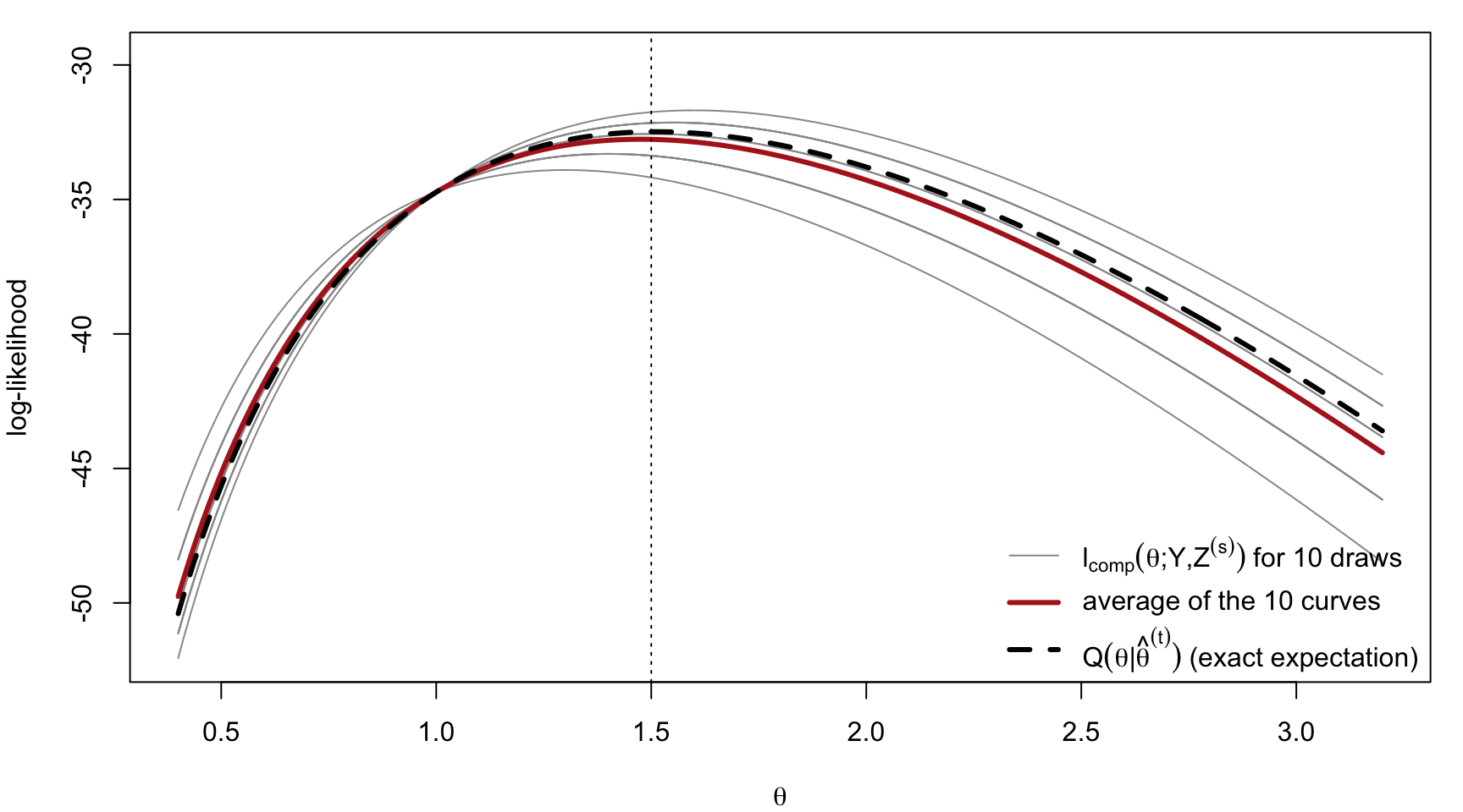
Fix \hat\theta^{(t)}. Each draw Z^{(s)}\sim P(Z\mid Y,\hat\theta^{(t)}) gives one curve \ell_{\text{comp}}(\theta;Y,Z^{(s)}); Q(\theta\mid\hat\theta^{(t)}) is their expectation (illustrated with the censored Poisson example of Section 3, \lambda^{(t)} = 1.5):
![]()
Kullback-Leibler Distance
Definition: for densities P(z) and q(z) on the same space, KL(P\|q) = \int P(z)\log\frac{P(z)}{q(z)}\,dz = E_P\!\left[\log\frac{P(Z)}{q(Z)}\right]
Theorem (Gibbs’ inequality): KL(P\|q) \ge 0, with equality iff P = q (a.e.)
Proof. Since \log x \le x - 1 (equality iff x=1),
\begin{aligned}
KL(P\|q) &= -\int P(z)\log\frac{q(z)}{P(z)}\,dz \ \ge\ -\int P(z)\Big(\frac{q(z)}{P(z)}-1\Big)\,dz \\
&= -\int\big[q(z)-P(z)\big]\,dz = 0 \qquad\blacksquare
\end{aligned}
Remarks:
- Measures how much q diverges from P; not symmetric (KL(P\|q)\ne KL(q\|P) in general).
- This inequality is what forces the H-term to decrease in the ascending-property proof (next slides), and what makes F(\tilde P,\theta) a lower bound on \ell_{\text{obs}}(\theta) later on
Simulation Check: E_P[\log P(X)] > E_P[\log q(X)]
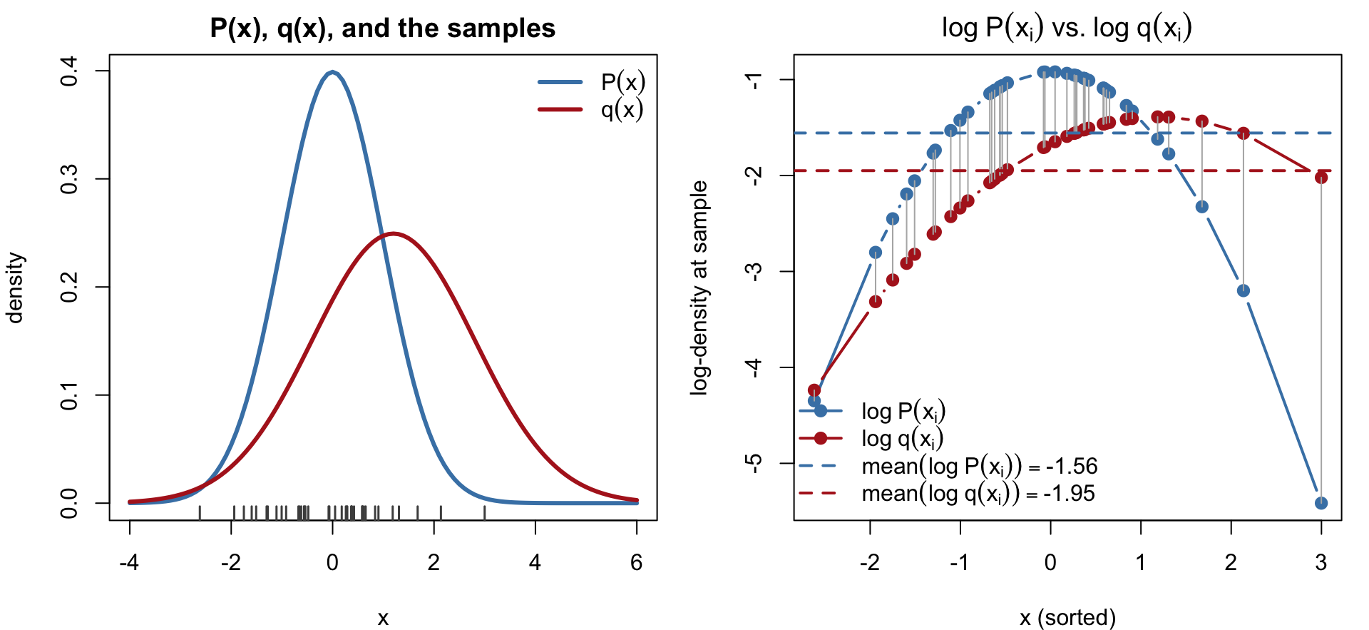
KL(P\|q) = E_P[\log P(X)] - E_P[\log q(X)] > 0 whenever q\ne P: draw x_1,\ldots,x_n\sim P and compare \log P(x_i) (blue) to \log q(x_i) (red) at the same sampled points.
![]()
- The blue dashed line (average of \log P(x_i)) always sits above the red one (average of \log q(x_i)); their gap is the (Monte Carlo estimate of the) KL(P\|q)
Ascending Property of EM
Write h(Y,Z\mid\theta) = P(Y,Z\mid\theta), \;g(Y\mid\theta) = \int h(Y,Z\mid\theta)\,dZ, \;K(Z\mid Y,\theta) = h/g.
Theorem. \;\ell_{\text{obs}}(\hat\theta^{(t+1)}) \ \ge\ \ell_{\text{obs}}(\hat\theta^{(t)}).
Key identity. Since \log g(Y\mid\theta) = \log h(Y,Z\mid\theta) - \log K(Z\mid Y,\theta) for every Z, taking E_{Z\mid Y,\theta_0} of both sides gives, for any \theta_0,
\ell_{\text{obs}}(\theta) = \underbrace{E_{Z\mid Y,\theta_0}\big[\log h(Y,Z\mid\theta)\big]}_{Q(\theta\mid\theta_0)}
- \underbrace{E_{Z\mid Y,\theta_0}\big[\log K(Z\mid Y,\theta)\big]}_{H(\theta\mid\theta_0)}
Intuition: maximizing Q makes the first term larger, and for any optimizer \theta the second term H (without the minus sign) is decreased — so \ell_{\text{obs}} is increased.
EM as Alternating Optimization
Let \tilde P(\cdot) be any distribution on the hidden data Z. Using P(Y,z\mid\theta) = P(Y\mid\theta)P(z\mid Y,\theta), we can define and express F(\tilde P,\theta) as:
\begin{aligned} F(\tilde P,\theta) &= \int \tilde P(z)\log P(Y,z\mid\theta)\,dz - \int \tilde P(z)\log\tilde P(z)\,dz \\ &= \ell_{\text{obs}}(\theta) - KL\big(\tilde P\,\Vert{}\,P(\cdot\mid Y,\theta)\big) \end{aligned}
where KL(P\Vert{}q) = \int P(z)\log\frac{P(z)}{q(z)}\,dz \ge 0.
- E-step = maximize F over \tilde P with \theta = \hat\theta^{(t)} fixed: KL \ge 0 with equality iff \tilde P = P(\cdot\mid Y,\hat\theta^{(t)}), so the E-step sets \tilde P to the conditional distribution of Z
- M-step = maximize F over \theta with \tilde P fixed: the second term of F is free of \theta, so this is \arg\max_\theta Q(\theta\mid\hat\theta^{(t)})
- Tight Bound = at \theta = \hat\theta^{(t)} (after the E-step), KL=0, meaning the lower bound exactly equals the observed log-likelihood: F(\tilde P,\hat\theta^{(t)}) = \ell_{\text{obs}}(\hat\theta^{(t)})
Q Functions as Tangent Lower Bounds
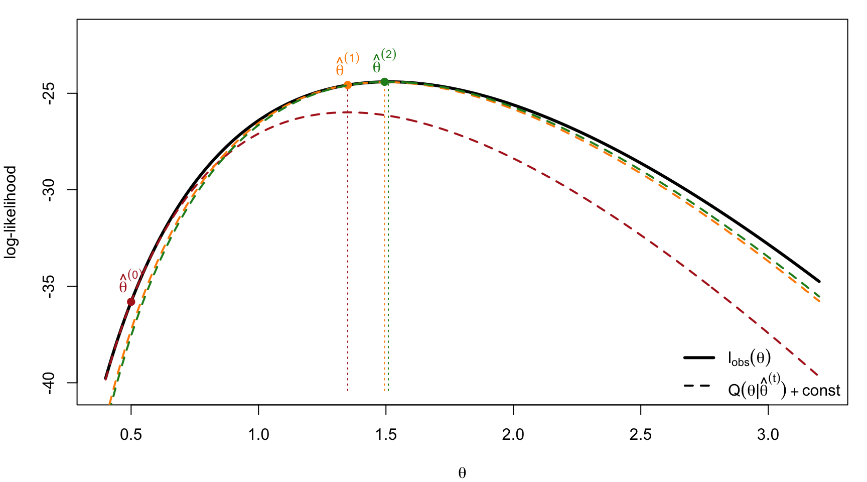
Each Q(\cdot\mid\hat\theta^{(t)}), shifted by a constant, lies below \ell_{\text{obs}} and touches it at \hat\theta^{(t)}; maximizing it moves uphill on \ell_{\text{obs}}.
![]()
2. Example 1: Two-Component Normal Mixture
Model and Likelihoods
Z_i \sim \text{Bern}(p), \qquad Y_i\mid Z_i = 1 \sim N(\mu_1,1), \qquad Y_i\mid Z_i = 0 \sim N(\mu_0,1)
Observed: y_1,\ldots,y_n. Hidden: z_1,\ldots,z_n. Parameter \theta = (\mu_0,\mu_1,p).
Complete likelihood P(y,z\mid\theta) = \prod_{i=1}^n P(y_i\mid z_i,\theta)\,P(z_i\mid\theta) = \prod_{i=1}^n \varphi(y_i\mid\mu_{z_i},1)\,p^{z_i}(1-p)^{1-z_i}
Observed likelihood (sum out each z_i) P(y\mid\theta) = \prod_{i=1}^n\Big[\varphi(y_i\mid\mu_1,1)\,p + \varphi(y_i\mid\mu_0,1)(1-p)\Big]
Model and Likelihoods (Continued)
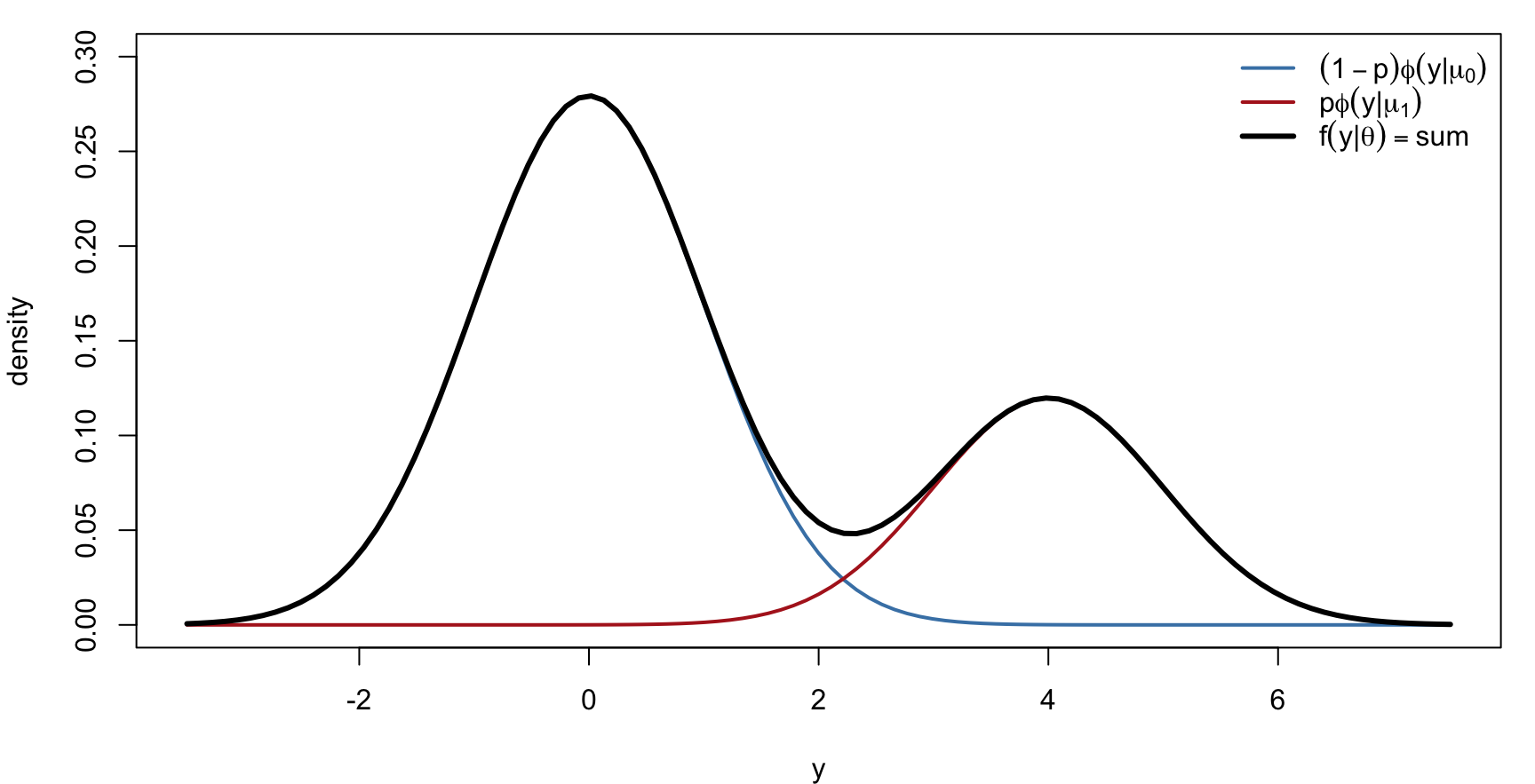
The observed likelihood is a product of mixture densities, each the sum of two weighted normal components:
![]()
The Mixture Density
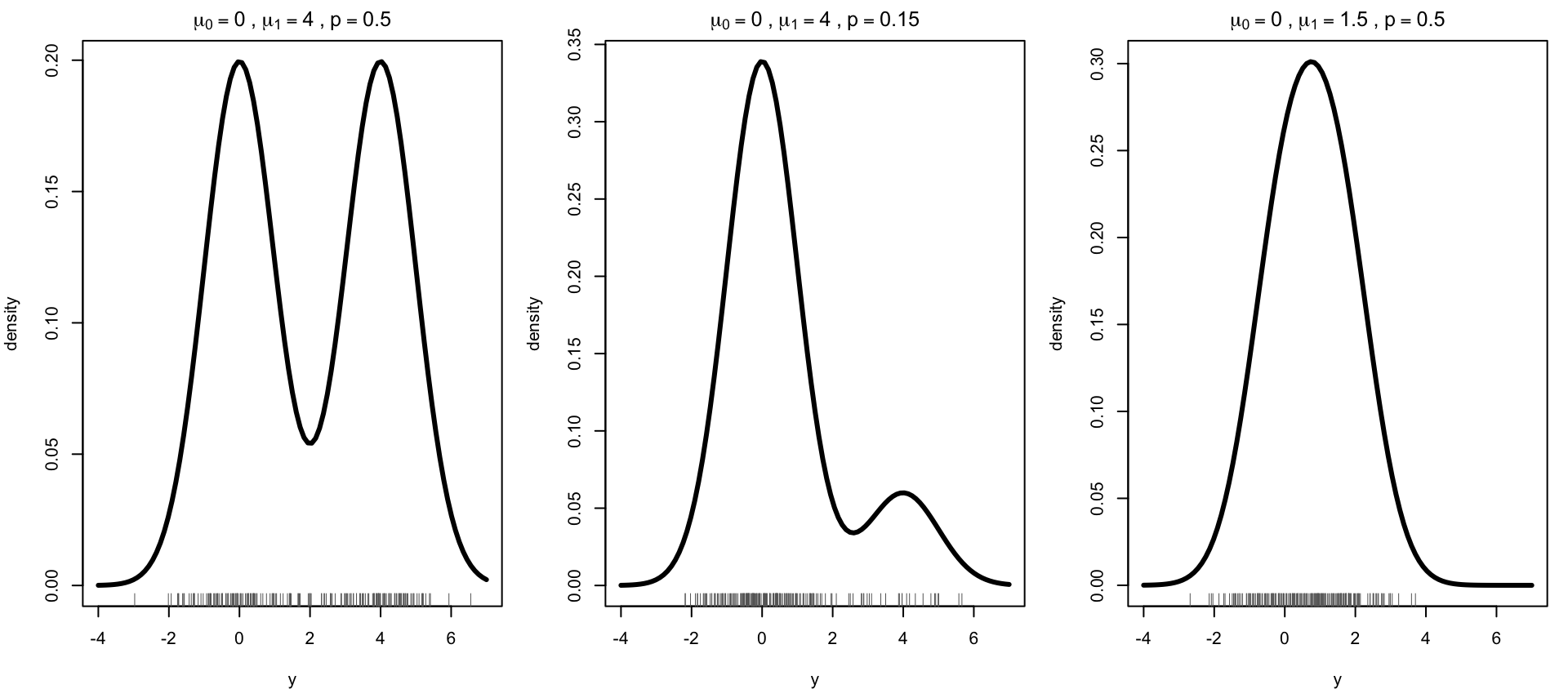
The marginal density f(y\mid\mu_0,\mu_1,p) can be bimodal or unimodal depending on p and |\mu_1-\mu_0|:
![]()
Maximizing \prod_i f(y_i\mid\theta) directly is awkward because of the sum inside the product; EM works with the complete likelihood instead.
Complete Log-Likelihood
With \log\varphi(y\mid\mu,1) = -\tfrac12(y-\mu)^2 - \log\sqrt{2\pi},
\begin{aligned}
\ell_{\text{comp}}(\theta;y,z)
&= \sum_{i=1}^n\Big[z_i\log p + (1-z_i)\log(1-p) - \tfrac12(y_i-\mu_{z_i})^2\Big] + C \\
&= \Big(\sum_{i=1}^n z_i\Big)\log\frac{p}{1-p} + n\log(1-p) \\
&\quad - \frac12\sum_{i=1}^n\Big[z_i(y_i-\mu_1)^2 + (1-z_i)(y_i-\mu_0)^2\Big] + C
\end{aligned}
- Linear in each z_i, so the E-step only needs E(Z_i\mid y_i,\hat\theta^{(t)})
- Given z, the parameters separate: p is a Bernoulli proportion, \mu_1,\mu_0 are group means
E-Step: Soft Classification
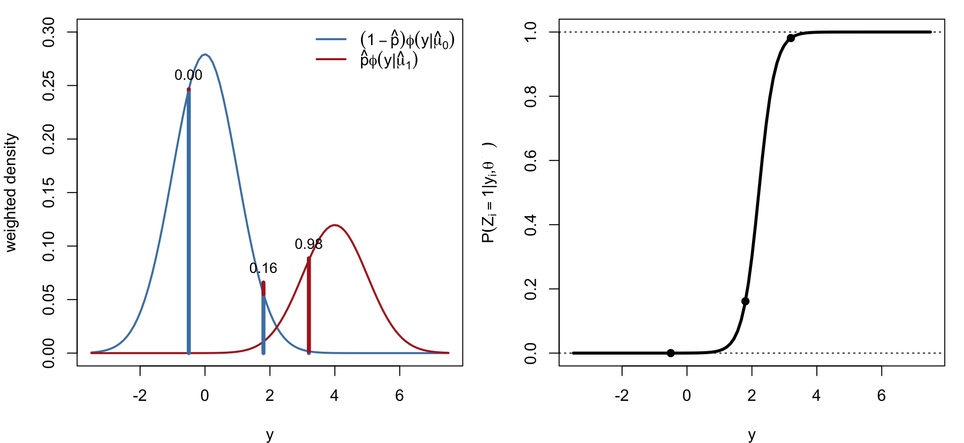
Given \hat\theta^{(t)} = (\hat\mu_0^{(t)},\hat\mu_1^{(t)},\hat p^{(t)}), Bayes’ rule gives
\hat p_i^{(t)} \equiv P(Z_i=1\mid y_i,\hat\theta^{(t)})
= \frac{\varphi(y_i\mid\hat\mu_1^{(t)},1)\,\hat p^{(t)}}
{\varphi(y_i\mid\hat\mu_0^{(t)},1)(1-\hat p^{(t)}) + \varphi(y_i\mid\hat\mu_1^{(t)},1)\,\hat p^{(t)}}
Then
\begin{aligned}
Q(\theta\mid\hat\theta^{(t)}) &= \Big(\sum_i \hat p_i^{(t)}\Big)\log\frac{p}{1-p} + n\log(1-p) \\
&\quad - \frac12\sum_i\Big[\hat p_i^{(t)}(y_i-\mu_1)^2 + (1-\hat p_i^{(t)})(y_i-\mu_0)^2\Big]
\end{aligned}
E-Step: Soft Classification (Continued)
Left: at each y_i, \hat p_i^{(t)} is the red share of the total height. Right: \hat p_i^{(t)} as a function of y_i.
![]()
M-Step: Weighted Proportions and Means
Q separates into a term in p and terms in \mu_1, \mu_0.
| p |
\dfrac{\partial Q}{\partial p} = \dfrac{\sum_i \hat p_i^{(t)}}{p(1-p)} - \dfrac{n}{1-p} = 0 \;\Longrightarrow\; \hat p^{(t+1)} = \dfrac1n\sum_{i=1}^n \hat p_i^{(t)} |
| \mu_1 |
\dfrac{\partial Q}{\partial \mu_1} = \sum_i \hat p_i^{(t)}(y_i-\mu_1) = 0 \;\Longrightarrow\; \hat\mu_1^{(t+1)} = \dfrac{\sum_i \hat p_i^{(t)}\,y_i}{\sum_i \hat p_i^{(t)}} |
| \mu_0 (weights 1-\hat p_i^{(t)}) |
\hat\mu_0^{(t+1)} = \dfrac{\sum_i (1-\hat p_i^{(t)})\,y_i}{\sum_i (1-\hat p_i^{(t)})} |
Return to the E-step with \hat\theta^{(t+1)} and recompute \hat p_i^{(t+1)}.
Interpretation: the M-step is the complete-data MLE with each observation split between the two groups according to its soft classification.
3. Example 2: Censored Poisson Data
Truncated Distributions in Brief
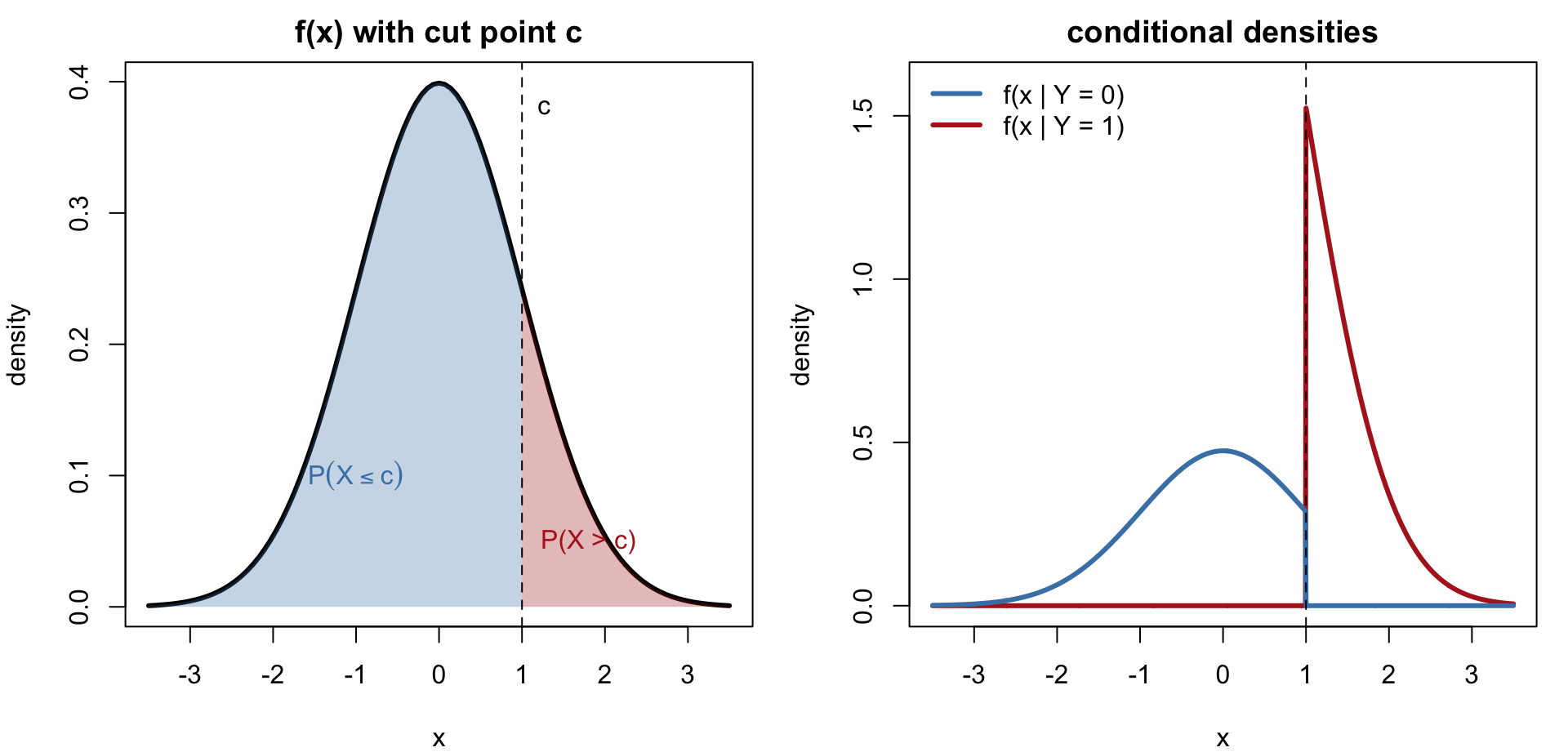
Let X\sim f(x) and Y = I(X>c). Then Y\sim\text{Bern}\big(P(X>c)\big), and the conditional distribution of X given Y is f restricted to one side of c and renormalized: f(x\mid Y=1) = \frac{f(x)\,I(x>c)}{\int_c^\infty f(t)\,dt}, \qquad
f(x\mid Y=0) = \frac{f(x)\,I(x\le c)}{\int_{-\infty}^c f(t)\,dt}
For discrete X the integrals are sums. This is exactly the distribution the E-step needs when an observation is only known to lie on one side of c.
Truncated Distributions in Brief (Continued)
![]()
Censored Poisson: Data and Likelihoods
y_i \overset{iid}{\sim}\text{Pois}(\lambda), i=1,\ldots,n. The first m values are observed exactly; for i>m we only know y_i<2, recorded as x_i = I(y_i<2) = 1.
Observed data: y_1,\ldots,y_m and x_{m+1}=\cdots=x_n=1. Missing: y_{m+1},\ldots,y_n.
Complete likelihood \prod_{i=1}^n f^{\text{Pois}}(y_i\mid\lambda)\cdot\prod_{i=m+1}^n I(y_i<2)
Observed likelihood \prod_{i=1}^m f^{\text{Pois}}(y_i\mid\lambda)\cdot\prod_{i=m+1}^n P(y_i<2\mid\lambda),
\qquad P(y_i<2\mid\lambda) = e^{-\lambda}(1+\lambda)
The second factor makes the MLE nonlinear in \lambda; EM sidesteps it.
E-Step
\ell_{\text{comp}}(\lambda) = -n\lambda + (\log\lambda)\sum_{i=1}^m y_i
+ (\log\lambda)\underbrace{\sum_{i=m+1}^n y_i}_{\text{missing}} - \sum_{i=1}^n\log(y_i!)
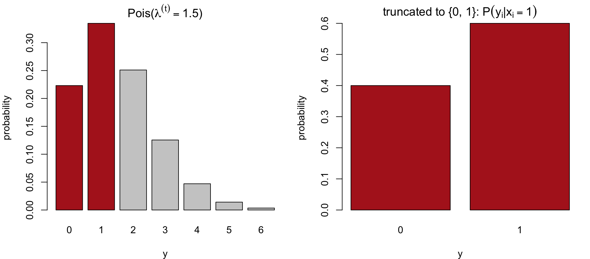
For i>m, y_i\in\{0,1\}, and the truncated Poisson given \lambda^{(t)} is P(y_i=0\mid x_i=1) = \frac{1}{1+\lambda^{(t)}}, \qquad P(y_i=1\mid x_i=1) = \frac{\lambda^{(t)}}{1+\lambda^{(t)}}
\hat y_i^{(t)} \equiv E(y_i\mid x_i=1,\lambda^{(t)}) = \frac{\lambda^{(t)}}{1+\lambda^{(t)}}
Since y_i! = 1 for y_i\in\{0,1\}, the \log(y_i!) term is a known constant and no further expectation is needed.
E-Step (Continued)
The conditional distribution of a censored y_i is the Poisson pmf restricted to \{0,1\} and renormalized:
![]()
M-Step and the EM Update
Q(\lambda\mid\lambda^{(t)}) = -n\lambda + (\log\lambda)\Big[\sum_{i=1}^m y_i + (n-m)\,\hat y^{(t)}\Big] + C^{(t)}
\frac{\partial Q}{\partial\lambda} = -n + \frac{1}{\lambda}\Big[\sum_{i=1}^m y_i + (n-m)\hat y^{(t)}\Big] = 0
\Longrightarrow\quad \lambda^{(t+1)} = \frac{m\,\bar y_{1:m} + (n-m)\dfrac{\lambda^{(t)}}{1+\lambda^{(t)}}}{n}
- The update is the ordinary Poisson MLE (sample mean) with each censored value replaced by its conditional expectation
- This works here only because \ell_{\text{comp}} is linear in the missing y_i; in general, EM is not “plug in E(Z) and maximize”
4. More Complex Applications
Model-Based Clustering
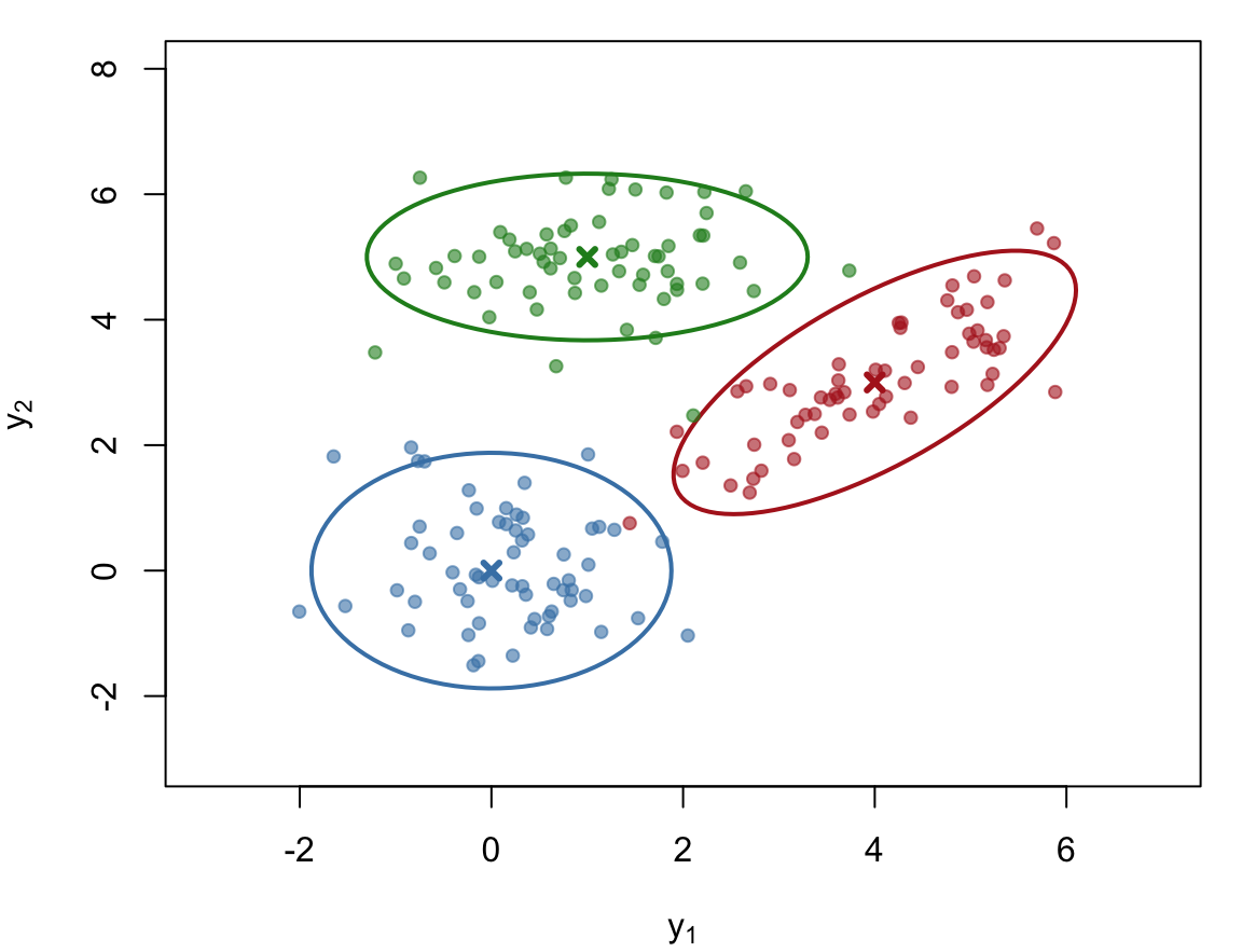
Z_i\sim\text{Categorical}(\pi_1,\ldots,\pi_K), \qquad Y_i\mid Z_i=k\sim N_d(\mu_k,\Sigma_k)
Multivariate, K-component generalization of Example 1. E-step: soft cluster memberships P(Z_i=k\mid y_i,\hat\theta^{(t)}); M-step: weighted means, covariances, and proportions.
![]()
Hidden Markov Models
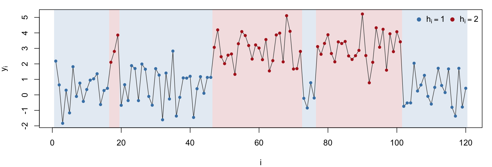
Hidden states h_1\to h_2\to\cdots\to h_n form a Markov chain; each observation depends only on its own state: P(y_{1:n}\mid h_{1:n},\theta) = \prod_{i=1}^n P(y_i\mid h_i,\theta)
E-step: the forward–backward algorithm computes P(h_i\mid y_{1:n},\hat\theta^{(t)}) and P(h_i,h_{i+1}\mid y_{1:n},\hat\theta^{(t)}) without enumerating all K^n state sequences. M-step: weighted transition and emission estimates (Baum–Welch).
![]()
Factor Analysis and the Common Pattern
Factor analysis y_i = \Gamma x_i + \varepsilon_i, \qquad x_i\sim N_q(0,I) \text{ hidden}, \quad \varepsilon_i\sim N_d(0,\Psi) E-step: x_i\mid y_i,\hat\theta^{(t)} is normal with closed-form mean and covariance. M-step: regression of y on the expected factors.
Common pattern across applications
- Introduce a hidden variable that makes the complete-data model tractable
- E-step: compute the conditional distribution (or expected sufficient statistics) of the hidden data
- M-step: complete-data MLE with the hidden data replaced by expected sufficient statistics
Summary
- EM maximizes \ell_{\text{obs}} by alternating between Q(\theta\mid\hat\theta^{(t)}) = E_{Z\mid Y,\hat\theta^{(t)}}[\ell_{\text{comp}}] and its maximizer
- Every iteration weakly increases \ell_{\text{obs}}; equivalently, EM is coordinate ascent on F(\tilde P,\theta) = \ell_{\text{obs}}(\theta) - KL\big(\tilde P\,\|\,P(Z\mid Y,\theta)\big)
- When \ell_{\text{comp}} is linear in sufficient statistics of Z, the E-step reduces to computing their conditional expectations
- Convergence is linear (often slow) and only to a stationary point; run from several starting values