Elements of Statistical Computation

Laplace Approximation

Longhai Li

2026-09-07

1. Goal and Idea

The Goal

Compute posterior expectations E_f\big[a(\theta)\big] = \frac{\int a(\theta)\,f(\theta)\,d\theta}{\int f(\theta)\,d\theta}

where

• a(\theta) is a function of \theta\in\mathbb R^p (a parameter, a prediction, an indicator)
• f(\theta) is the unnormalized posterior, e.g. f(\theta) = L(\theta)\,\pi(\theta), or a penalized likelihood
• both numerator and denominator are p-dimensional integrals

Quadrature works only for small p; Monte Carlo needs a sampler. The Laplace approximation replaces the integrals by a closed-form Gaussian integral, exploiting the fact that for large n the posterior is nearly normal.

The Idea

Write the negative log unnormalized posterior h(\theta) = -\log f(\theta), \qquad f(\theta) = e^{-h(\theta)}

• h is (up to a constant) the negative log-likelihood plus the negative log-prior: a sum of n terms, so it grows like n and becomes sharply curved at its minimum
• When n is large, \theta\mid\text{data} \ \approx\ N\big(\hat\theta_0,\ \hat\Sigma_0\big) with \hat\theta_0 the posterior mode and \hat\Sigma_0 determined by the curvature of h there

The approximation is obtained by expanding h to second order around its minimum and integrating the resulting Gaussian exactly.

2. Derivation

Second-Order Taylor Expansion

Let \theta_0 = \arg\min_\theta h(\theta) (the posterior mode), found by optimization. Expand h around \theta_0: h(\theta) = h(\theta_0) + \underbrace{\nabla h(\theta_0)^\top}_{=\,0 \text{ at the minimum}}(\theta-\theta_0) + \tfrac12(\theta-\theta_0)^\top\nabla^2 h(\theta_0)(\theta-\theta_0) + O\big(\|\theta-\theta_0\|^3\big)

Keeping terms up to second order, h(\theta)\ \approx\ \tilde h(\theta) = h(\theta_0) + \tfrac12(\theta-\theta_0)^\top H\,(\theta-\theta_0), H = \nabla^2 h(\theta_0)

• H is the Hessian of -\log f at the mode; it is positive definite at a strict minimum
• For f = L\pi, H is the observed information plus the prior curvature

From \tilde h to a Gaussian

\begin{aligned} f(\theta)\ \approx\ \tilde f(\theta) &= e^{-\tilde h(\theta)} = e^{-h(\theta_0)}\cdot\exp\Big\{-\tfrac12(\theta-\theta_0)^\top H(\theta-\theta_0)\Big\} \\[4pt] &= \underbrace{f(\theta_0)\,(2\pi)^{p/2}\,|H|^{-1/2}}_{\text{constant}} \cdot\underbrace{(2\pi)^{-p/2}\,|H|^{1/2}\exp\Big\{-\tfrac12(\theta-\theta_0)^\top H(\theta-\theta_0)\Big\}}_{N_p(\theta_0,\,H^{-1})\text{ density, integrates to }1} \end{aligned}

Review: if X\sim N_p(\mu,\Sigma), then p(x) = (2\pi)^{-p/2}|\Sigma|^{-1/2}\exp\{-\tfrac12(x-\mu)^\top\Sigma^{-1}(x-\mu)\}. Here \Sigma = H^{-1}, so |\Sigma|^{-1/2} = |H|^{1/2}.

The Two Results

1. Posterior approximation \theta\mid\text{data}\ \approx\ N_p\Big(\theta_0,\ \big[\nabla^2 h(\theta_0)\big]^{-1}\Big)

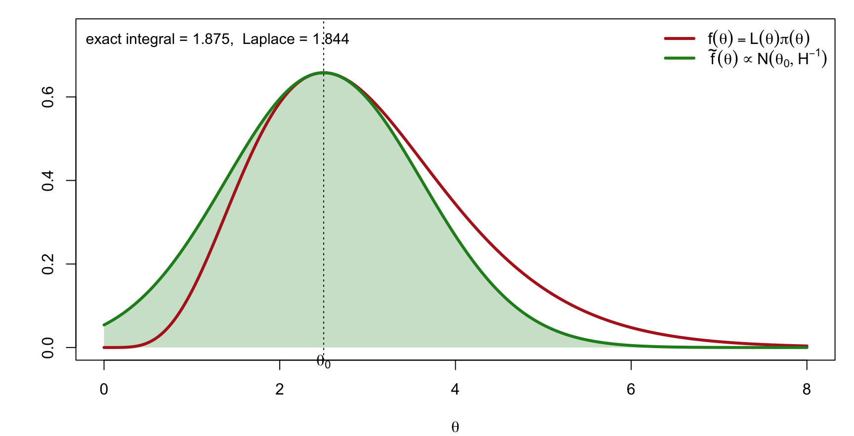
2. Normalizing constant (marginal likelihood) \int f(\theta)\,d\theta\ \approx\ f(\theta_0)\,(2\pi)^{p/2}\,\big|\nabla^2 h(\theta_0)\big|^{-1/2}

Only two ingredients are needed: the mode \theta_0 and the Hessian of -\log f at the mode, both available from a numerical optimizer (optim(..., hessian = TRUE) in R).

The relative error of (2) is O(1/n) for regular models; the error of (1) is driven by the skewness of the true posterior.

The Two Results (Continued)

Red: unnormalized posterior f(\theta). Green: the Gaussian \tilde f(\theta) matching height and curvature at the mode. The shaded rectangle-like region has area f(\theta_0)(2\pi)^{p/2}|H|^{-1/2}, the Laplace estimate of \int f(\theta)\,d\theta.

3. Applications

Application 1: Marginal Likelihood and BIC

With f(\theta) = L(\theta;D)\,\pi(\theta), the marginal likelihood P(D) = \int L(\theta;D)\pi(\theta)\,d\theta satisfies \log P(D)\ \approx\ \log\big[P(D\mid\theta_0)\,\pi(\theta_0)\big] + \frac p2\log(2\pi) - \frac12\log\big|\nabla^2 h(\theta_0)\big|

Simplification for large n. The Hessian is dominated by the likelihood: \nabla^2 h(\theta_0)\approx n\,I(\theta_0) with I the per-observation Fisher information, so |\nabla^2 h(\theta_0)| \approx n^p\,|I(\theta_0)| and \log P(D) \approx \log P(D\mid\theta_0) - \frac p2\log n + \underbrace{\log\pi(\theta_0) + \frac p2\log(2\pi) - \frac12\log|I(\theta_0)|}_{O(1),\ \text{dropped}}

Multiplying by -2 and replacing the posterior mode by the MLE gives the Bayesian information criterion: \text{BIC} = -2\log L(\hat\theta_{\text{MLE}}) + p\log n

Application 2: Linear Functions of \theta

If a(\theta) = A^\top\theta + a_0 is linear, replace f by its Gaussian approximation: E_f\big[a(\theta)\big]\ \approx\ E_{\tilde f}\big[a(\theta)\big] = A^\top E_{\tilde f}(\theta) + a_0 = A^\top\theta_0 + a_0

• The posterior mean is approximated by the posterior mode
• Posterior variances and covariances come from H^{-1}: \text{Var}_{\tilde f}(A^\top\theta) = A^\top H^{-1}A
• Credible intervals: \theta_{0j}\pm z_{\alpha/2}\sqrt{(H^{-1})_{jj}}

This is exactly the Bayesian counterpart of MLE plus Wald standard errors.

Example: Poisson Rate with a Gamma Prior

y_1,\ldots,y_n\mid\lambda\sim\text{Pois}(\lambda), \lambda\sim\text{Gamma}(\alpha,\beta). The posterior is \text{Gamma}(\alpha+\sum y_i,\ \beta+n) and P(y) is available exactly, so we can measure the Laplace error.

alpha <- 2; beta <- 1
laplace_ml <- function(y) { n <- length(y); s <- sum(y)
  h  <- function(l) -(sum(dpois(y, l, log = TRUE)) + dgamma(l, alpha, beta, log = TRUE))
  op <- optim(mean(y) + 0.5, h, method = "L-BFGS-B", lower = 1e-6, hessian = TRUE)
  c(mode = op$par, log_ml = -op$value + 0.5 * log(2 * pi) - 0.5 * log(op$hessian[1, 1])) }
exact_log_ml <- function(y) { n <- length(y); s <- sum(y)
  alpha * log(beta) - lgamma(alpha) + lgamma(alpha + s) - (alpha + s) * log(beta + n) - sum(lfactorial(y)) }
res <- t(sapply(c(5, 20, 100, 500), function(n) { y <- rpois(n, 3)
  c(n = n, laplace_ml(y), exact = exact_log_ml(y), post_mean = (alpha + sum(y)) / (beta + n)) }))
round(cbind(res, error = res[, "log_ml"] - res[, "exact"]), 4)

       n   mode    log_ml     exact post_mean   error
[1,]   5 2.5000  -11.0017  -10.9962    2.6667 -0.0056
[2,]  20 2.8095  -38.8421  -38.8407    2.8571 -0.0014
[3,] 100 2.9802 -201.4952 -201.4950    2.9901 -0.0003
[4,] 500 2.9321 -957.8226 -957.8225    2.9341 -0.0001

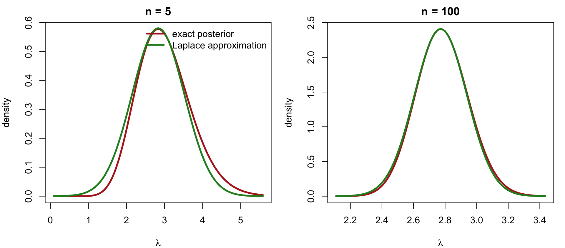
The error in \log P(y) shrinks roughly like 1/n, and the mode approaches the posterior mean as the Gamma posterior becomes symmetric.

Example (Continued)

Exact Gamma posterior (red) and the Laplace normal approximation (green) for n = 5 and n = 100.

When Laplace Works Well, and When It Does Not

Works well

• Large n relative to p, unimodal and roughly symmetric posterior
• Parameters on an unbounded scale: transform first (\log\sigma, \text{logit}\,p) so the Gaussian is not truncated at a boundary; the Jacobian must then be included in f

Problems

• Skewed posteriors (small n, parameters near a boundary): the mode is a poor centre and tails are wrong
• Multimodal posteriors: only the mode found is represented
• Hierarchical models with many parameters: p grows with n, so the O(1/n) error does not vanish; nested Laplace (INLA) integrates out the high-dimensional part analytically

Summary

• Laplace approximation: expand h = -\log f to second order at its minimum \theta_0 and integrate the Gaussian exactly \theta\mid\text{data}\approx N_p\big(\theta_0, [\nabla^2h(\theta_0)]^{-1}\big), \int f(\theta)\,d\theta \approx f(\theta_0)(2\pi)^{p/2}|\nabla^2 h(\theta_0)|^{-1/2}
• Needs only an optimizer and a Hessian; cost does not grow with the number of integrals
• Gives BIC as a large-n simplification of the marginal likelihood
• Linear a(\theta): mode and H^{-1} suffice; general a(\theta): simulate from the Gaussian or use two Laplace approximations
• Deterministic, fast, and accurate to O(1/n), but blind to skewness and multimodality; Monte Carlo methods (next lectures) remove these limitations at higher computational cost