Elements of Statistical Computation

Importance Sampling

Longhai Li

2026-10-06

1. Goal and Idea

The Goal

Rejection sampling turns draws from an envelope g\ge f into exact draws from f, but every rejected proposal is wasted — and in the tails of a poor envelope, almost every proposal is rejected.

Two integrals with respect to an unnormalized function f(\theta), e.g. f(\theta) = \pi(\theta)L(\theta):

  1. A posterior expectation. A = \frac{\int a(\theta)\,f(\theta)\,d\theta}{\int f(\theta)\,d\theta} = E_f\big[a(\theta)\big], \qquad \theta\sim\frac{f(\theta)}{C_f}

  2. The normalizing constant (marginal likelihood). C_f = \int f(\theta)\,d\theta.

Plain Monte Carlo needs draws from f/C_f, which we cannot produce. Rejection sampling needs an envelope g\ge f, which may be hard to find or very wasteful.

The Idea: Reweighting

Importance sampling keeps every proposal instead of discarding most of them: draw from an easier function g and attach a weight that corrects for sampling from the wrong distribution. Nothing is ever thrown away, and no envelope condition g\ge f is required — the price is that the sample is no longer an exact iid sample from f, only a weighted one.

  • Draw \theta\sim g(\theta)/C_g, where g is another (possibly unnormalized) function we can sample from

  • Attach the importance weight, w(\theta) = \frac{f(\theta)}{g(\theta)}

  • Hope that w(\theta)\approx constant, i.e. g has roughly the shape of f

Requirement on g: wherever f is positive, g must be positive too, \{\theta: g(\theta)>0\}\ \supseteq\ \{\theta: f(\theta)>0\}.

Otherwise part of f is never visited and the estimate is biased (Example 2).

2. The Importance Reweighting Formula

Derivation

Let C_g = \int g(\theta)\,d\theta. For any a, \begin{aligned} E_f\big[a(\theta)\big] &= \int a(\theta)\,\frac{f(\theta)}{C_f}\,d\theta = \frac{C_g}{C_f}\int a(\theta)\,\frac{f(\theta)}{g(\theta)}\cdot\frac{g(\theta)}{C_g}\,d\theta \\[4pt] &= \frac{C_g}{C_f}\,E_g\big[a(\theta)\,w(\theta)\big], \qquad w(\theta) = \frac{f(\theta)}{g(\theta)}. \end{aligned}

The division by g is legitimate only on \{g>0\}, hence the support requirement.

Taking a\equiv1, \frac{C_f}{C_g} = \int\frac{f(\theta)}{g(\theta)}\cdot\frac{g(\theta)}{C_g}\,d\theta = E_g\big[w(\theta)\big] = \frac{\int f(\theta)\,d\theta}{\int g(\theta)\,d\theta}.

Combining, E_f\big[a(\theta)\big] = \frac{E_g\big[a(\theta)\,w(\theta)\big]}{E_g\big[w(\theta)\big]}.

The Estimators

Draw \theta_1,\ldots,\theta_{\mathrm{S}} \overset{iid}{\sim} g/C_g and compute w_s = w(\theta_s) = f(\theta_s)/g(\theta_s).

Ratio of normalizing constants \widehat{\frac{C_f}{C_g}} = \frac1S\sum_{s=1}^S w_s.

Unbiased for C_f/C_g; if g is a normalized density (C_g=1) this estimates C_f itself — e.g. the marginal likelihood.

Self-normalized expectation \hat A = \frac{\frac1S\sum_s a(\theta_s)\,w_s}{\frac1S\sum_s w_s} = \sum_{s=1}^S a(\theta_s)\,\tilde w_s, \qquad \tilde w_s = \frac{w_s}{\sum_{j=1}^S w_j}, \quad \sum_s\tilde w_s = 1

\tilde w_s turns the proposal sample into a weighted sample from f; unknown constants in f and g cancel. It is a ratio of two averages, so it is biased with bias O(1/S), but consistent.

Effective Sample Size

How many “equally informative” draws is a weighted sample worth?. S_{\text{eff}} = \frac{1}{\sum_{s=1}^S \tilde w_s^2}.

If w_s\approx constant (proposal shaped like the target), \tilde w_s = 1/S and S_{\text{eff}} = S: full efficiency. If one weight dominates, S_{\text{eff}}\approx1: only one draw is doing any work.

Variance heuristic: \operatorname{Var}_g(\hat A)\approx\operatorname{Var}_f(a)/S_{\text{eff}}, the same form as for an iid sample of size S_{\text{eff}} from f itself.

The catch, central to this lecture: S_{\text{eff}} is computed only from the weights actually observed. A proposal that never visits the part of \theta-space where f and g disagree most will report a reassuring S_{\text{eff}} while being badly wrong.

Where the ESS Formula Comes From

Write \hat A = \overline N/\overline D with N_s = w_s a(\theta_s), D_s = w_s. The delta method gives \operatorname{Var}_g(\hat A) \approx \frac{1}{S}E_g\!\bigl[w^{2}(a-A)^{2}\bigr] = \frac{1}{S}E_f\!\bigl[w(a-A)^{2}\bigr], using E_g[w\,h] = E_f[h]. If w varies little across the support of (a-A)^2, this factors as E_g[w^2]\operatorname{Var}_f(a)/S, giving \operatorname{Var}_g(\hat A) \approx \frac{\operatorname{Var}_f(a)}{S_{\text{eff}}^{\star}}, \qquad S_{\text{eff}}^{\star} := \frac{S}{E_g[w^{2}]}

S_{\text{eff}}^{\star} is a property of f and g alone — independent of a or the sample — and it is the metric that reveals pathologies (missed modes, heavy tails) even when the observed S_{\text{eff}} looks fine.

Plugging in sample moments, \frac{1}{S}\sum w_s for E_g[w] and \frac{1}{S}\sum w_s^2 for E_g[w^2], turns S_{\text{eff}}^\star into Kish’s formula (\sum w_s)^2/\sum w_s^2 = 1/\sum\tilde w_s^2 — a principled plug-in estimator, not an ad hoc heuristic.

Limitations of the ESS Diagnostic

Kish’s approximation is not uniformly precise. With f=N(0,1), g=N(0,2^2), a(\theta)=\theta^2, S=4000:

  • empirical \operatorname{Var}(\hat A)\approx 3.15\times10^{-4}, matching exact delta-method calculations

  • but \operatorname{Var}_f(a)/S_{\text{eff}}^\star \approx 7.56\times10^{-4} — over twice as large, because w and (a-A)^2 are negatively correlated here

More critically: \widehat{S_{\text{eff}}} is computed only from the observed weights. If the proposal never explores where f and g disagree most, the estimator reports a falsely reassuring \widehat{S_{\text{eff}}} and masks a severe sampling inadequacy — the subject of Examples 1 and 2 below.

3. Example 1: Same Support, but a Mode Is Missed

Example 1: Same Support, but a Mode Is Missed,

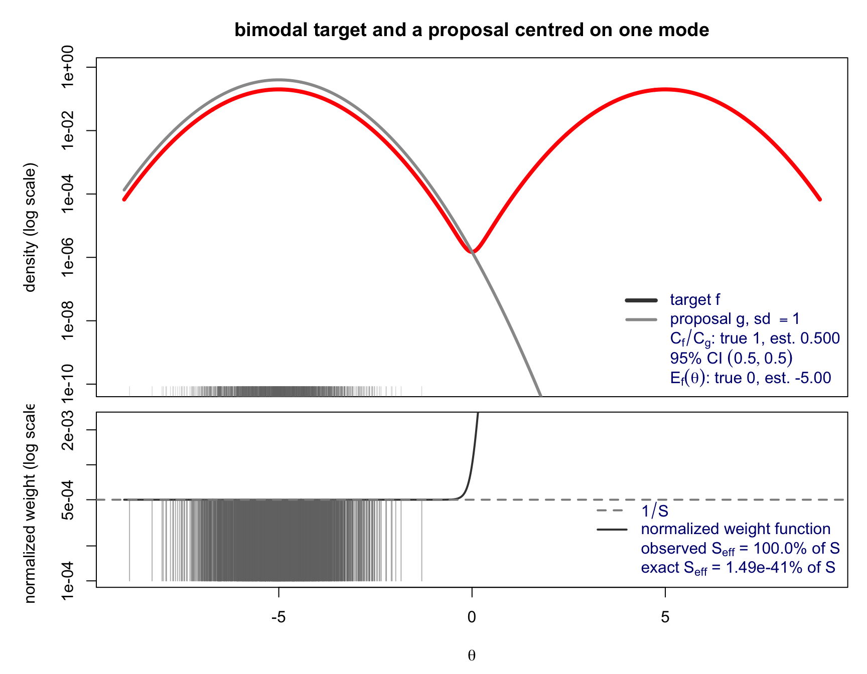
f(\theta) = \tfrac12\varphi(\theta+d) + \tfrac12\varphi(\theta-d), \qquad g_{\sigma}(\theta) = \tfrac{1}{\sigma}\varphi\!\left(\tfrac{\theta+d}{\sigma}\right), \qquad d = 5.

Both are positive on all of \mathbb{R}, so the support requirement holds. But for \sigma of order one the proposal concentrates around -d and never produces draws near the second mode at +d.

For \theta near -d and \sigma=1, w(\theta) = \tfrac12 + \tfrac12\,\frac{\varphi(\theta-d)}{\varphi(\theta+d)} = \tfrac12 + \tfrac12 e^{2d\theta} \;\approx\; \tfrac12,

so every observed weight is nearly equal, \tilde w_i\approx1/S and S_{\text{eff}}\approx S, while \widehat{C_f/C_g}\approx\tfrac12 (truth 1) and \hat E_f(\theta)\approx-d (truth 0). The draws that would expose the error carry w\approx\tfrac12e^{2d\theta}\gg1 near \theta=+d and have probability \Phi(-2d)\approx10^{-23} under g_1: they never appear.

Example 1 (Continued): The Figure

Figure 1

The observed effective sample size reports near-perfect efficiency. The exact effective fraction 1/E_g(w^2) is smaller by forty orders of magnitude — a property of f,g alone, invisible to any single sample. The variance is finite at \sigma=1 (it diverges only for \sigma\le1/\sqrt2), so the estimator is consistent — it would just need S\sim10^{43} to look normal.

4. Example 2: Tail Probability of a Student-t Distribution

Example 2: Tail Probability of a Student-t Distribution

The target is a standard Student-t_\nu: \nu=1 is the Cauchy, \nu\to\infty recovers the normal — \nu is a tuning parameter of the target’s tail weight. Goal: P(c_1<X<c_2) for an interval (c_1,c_2), possibly one-sided (c_2=\infty), from a truncated-normal proposal sampled by adaptive rejection sampling (ARS).

\log\varphi is concave, and restricting to (c_1,c_2) preserves concavity, so the ars package applies directly to the proposal.

Code
rtnorm_ars <- function(n, mu = 0, sigma = 1, lo = 0, hi = Inf) {
    logf   <- function(x) dnorm(x, mu, sigma, log = TRUE)
    fprima <- function(x) -(x - mu) / sigma^2
    if (is.finite(hi)) {
        x0 <- lo + (hi - lo) * c(0.1, 0.5, 0.9)
    } else {
        right <- max(mu, lo) + 3 * sigma
        x0 <- sort(unique(c(lo + 0.1 * sigma, max(lo + 0.2 * sigma, mu + 1e-6), right)))
    }
    ars(n, f = logf, fprima = fprima, x = x0,
        lb = TRUE, xlb = lo, ub = is.finite(hi), xub = if (is.finite(hi)) hi else 0)
}

The target \log f_{t_\nu} is not concave at any finite \nu — convex out in the tails, concave everywhere only in the \nu\to\infty limit — so ARS cannot sample it directly. The truncated-normal proposal is a substitute, which is exactly why the sample needs importance weights.

Example 2 (Continued): The Estimator

Let g be the normalized truncated normal on (c_1,c_2), f(x)=f_{t_\nu}(x)I(c_1<x<c_2). Draw X_1,\ldots,X_{\mathrm{S}}\sim g, weight by w=f/g, average: \widehat C = \frac1S\sum_{i=1}^S w(X_i), unbiased for C_f=P(c_1<X<c_2) for any g positive wherever f is — regardless of c_1,c_2,\mu,\sigma,\nu.

Example 2 (Continued): When Its Variance Is Infinite

Precision is a different question: \operatorname{Var}_g\bigl(w(X)\bigr) = \int_{c_1}^{c_2}\frac{f_{t_\nu}(x)^2}{g(x)}\,dx - C_f^2

  • c_2 finite: f,g share the same bounded interval, f/g is bounded on it, the integral is finite — well-behaved at any \nu.

  • c_2\to\infty: f_{t_\nu}(x)^2 decays only polynomially (\propto x^{-2(\nu+1)}), g’s Gaussian tail decays much faster — the integrand grows without bound and the integral diverges, for every \mu,\sigma and every finite \nu.

S_{\text{eff}} need not warn you which regime you are in.

Example 2 (Continued): is_t_interval()

Code
is_t_interval <- function(S, df, c1, c2, mu, sigma, seed = NULL) {
    if (!is.null(seed)) set.seed(seed)
    X <- rtnorm_ars(S, mu, sigma, c1, c2)

    lZ   <- log(pnorm(c2, mu, sigma) - pnorm(c1, mu, sigma))
    logw <- dt(X, df, log = TRUE) - (dnorm(X, mu, sigma, log = TRUE) - lZ)

    m    <- max(logw); v <- exp(logw - m)
    Chat <- mean(v) * exp(m); se <- sd(v) / sqrt(S) * exp(m)
    wn   <- v / sum(v)

    list(X = X, wn = wn, Chat = Chat, se = se, ess = 1 / sum(wn^2),
         truth = pt(c2, df) - pt(c1, df))
}
Code
settings <- data.frame(df = c(1, 10, 1, 30), c1 = c(1, 1, 1, 1), c2 = c(3, 3, Inf, Inf))
res <- lapply(seq_len(nrow(settings)), function(i) with(settings[i, ],
    is_t_interval(S = 5000, df = df, c1 = c1, c2 = c2, mu = 0, sigma = 1, seed = 1)))

knitr::kable(data.frame(
    df = settings$df, c1 = settings$c1,
    c2 = ifelse(is.finite(settings$c2), as.character(settings$c2), "Inf"),
    truth = sapply(res, `[[`, "truth"), estimate = sapply(res, `[[`, "Chat"),
    se = sapply(res, `[[`, "se"), ess_pct = 100 * sapply(res, `[[`, "ess") / 5000
), digits = 4, col.names = c("df", "c1", "c2", "truth", "estimate", "s.e.", "ESS %"))
Table 1
df c1 c2 truth estimate s.e. ESS %
1 1 3 0.1476 0.1490 0.0014 68.7656
10 1 3 0.1638 0.1642 0.0004 96.8918
1 1 Inf 0.2500 0.1821 0.0128 3.9146
30 1 Inf 0.1627 0.1627 0.0003 98.5371

A finite interval is well-behaved at any \nu; c_2=\infty reproduces the divergence — badly at \nu=1, only deceptively well at \nu=30.

Example 2 (Continued):Observations

  • c_2 finite (default): weights have finite variance; raising S improves the estimate at the usual 1/\sqrt S rate, and the 95% interval covers about as often as claimed

  • Check “c_2=\infty”: reproduces the divergent case. Raising S no longer shrinks a variance that doesn’t exist; repeated New sample draws swing far more than the SE admits. Large \nu can still look fine by chance; small \nu (Cauchy) bites often — but S_{\text{eff}} warns you either way only sometimes

  • Small \sigma, or \mu far outside (c_1,c_2): draws pile up wherever the proposal has mass, weights nearly equal, S_{\text{eff}} stays high, estimate can still miss badly

  • Large \sigma: one draw’s weight can dominate, S_{\text{eff}} collapses toward 1 — visibly unreliable, an improvement on invisibly unreliable

5. Example 3: Marginal Likelihood via Importance Sampling

Example 3: Marginal Likelihood via Importance Sampling

Model: unknown mean \mu and w=\log\sigma^2, independent normal priors. Importance sampling estimates P(y)=\int L(\theta)\pi(\theta)\,d\theta with a built-in diagnostic (S_{\text{eff}}).

Take g(\mu,w) to be the Gaussian approximation to the posterior from a Laplace fit: mode (\hat\mu,\hat w), g=N_2\big((\hat\mu,\hat w), H^{-1}\big) for H the Hessian of -\log[L\pi] at the mode: \widehat{P(y)} = \frac1S\sum_{s=1}^S w_s, \qquad w_s = \frac{L(\theta_s)\pi(\theta_s)}{g(\theta_s)}, \qquad \theta_s\sim g.

Contrast: sampling directly from the (wide, uninformative) prior is importance sampling with g=\pi and weights L(\theta_s) — a “good story” versus a proposal built with no information about where the likelihood actually lives.

Example 3 (Continued): Implementation

log_lik   <- function(x, mu, w) sum(dnorm(x, mu, exp(w / 2), log = TRUE))
log_prior <- function(mu, w, mu_0, sigma_mu, w_0, sigma_w) {
    dnorm(mu, mu_0, sigma_mu, log = TRUE) + dnorm(w, w_0, sigma_w, log = TRUE)
}
neg_log_post <- function(theta, x, mu_0, sigma_mu, w_0, sigma_w) {
    -log_lik(x, theta[1], theta[2]) -
        log_prior(theta[1], theta[2], mu_0, sigma_mu, w_0, sigma_w)
}
log_dmvnorm_batch <- function(Theta, mu, A) {           # log N(mu, A^-1) at every column at once
    Tc <- Theta - mu
    quad <- colSums((A %*% Tc) * Tc)
    0.5 * (-nrow(Theta) * log(2 * pi) + sum(log(svd(A)$d)) - quad)
}
log_marlik_imps <- function(x, mu_0, sigma_mu, w_0, sigma_w, S) {
    fit <- nlm(neg_log_post, c(mean(x), log(stats::var(x))), hessian = TRUE,
               x = x, mu_0 = mu_0, sigma_mu = sigma_mu, w_0 = w_0, sigma_w = sigma_w)
    mu_hat <- fit$estimate; H <- fit$hessian
    L <- t(chol(solve(H)))
    Theta <- L %*% matrix(rnorm(2 * S), 2, S) + mu_hat
    log_g <- log_dmvnorm_batch(Theta, mu_hat, H)
    log_f <- -apply(Theta, 2, neg_log_post, x = x, mu_0 = mu_0, sigma_mu = sigma_mu,
                     w_0 = w_0, sigma_w = sigma_w)
    lw <- log_f - log_g
    m  <- max(lw); v <- exp(lw - m)
    structure(log_sum_exp(lw) - log(S), ess = log_ess(lw), se = sd(v) / (sqrt(S) * mean(v)))
}
log_marlik_prior <- function(x, mu_0, sigma_mu, w_0, sigma_w, S) {
    mus <- rnorm(S, mu_0, sigma_mu); ws <- rnorm(S, w_0, sigma_w)
    lw <- vapply(seq_len(S), function(i) log_lik(x, mus[i], ws[i]), numeric(1))
    m  <- max(lw); v <- exp(lw - m)
    structure(log_sum_exp(lw) - log(S), ess = log_ess(lw), se = sd(v) / (sqrt(S) * mean(v)))
}
log_marlik_grid <- function(x, mu_0, sigma_mu, w_0, sigma_w, n_grid = 400, width = 8) {
    n   <- length(x)
    fit <- nlm(neg_log_post, c(mean(x), log(stats::var(x))), hessian = TRUE,
               x = x, mu_0 = mu_0, sigma_mu = sigma_mu, w_0 = w_0, sigma_w = sigma_w)
    se  <- sqrt(diag(solve(fit$hessian)))
    mu_grid <- fit$estimate[1] + seq(-width, width, length.out = n_grid) * se[1]
    w_grid  <- fit$estimate[2] + seq(-width, width, length.out = n_grid) * se[2]
    SS <- sum(x^2) - 2 * mu_grid * sum(x) + n * mu_grid^2
    log_lik_grid   <- outer(SS, w_grid,
                             function(ss, w) -0.5 * n * log(2 * pi) - n * w / 2 - 0.5 * exp(-w) * ss)
    log_prior_grid <- outer(dnorm(mu_grid, mu_0, sigma_mu, log = TRUE),
                             dnorm(w_grid, w_0, sigma_w, log = TRUE), "+")
    h_mu <- diff(mu_grid[1:2]); h_w <- diff(w_grid[1:2])
    log_sum_exp(as.vector(log_lik_grid + log_prior_grid)) + log(h_mu) + log(h_w)
}
log_marlik_grid() supplies ground truth by quadrature — a midpoint grid centred and scaled by the Laplace fit, vectorized via the sufficient statistic \sum(x-\mu)^2.

Example 3 (Continued): Results Across Sample Sizes

Code
set.seed(4)
ns <- c(5, 20, 100, 400); S <- 2000

summarize_is <- function(fn, x, S) {
    est <- fn(x, 0, 5, 0, 5, S); se <- attr(est, "se")
    c(estimate = sprintf("%.2f", as.numeric(est)),
      ci       = sprintf("(%.2f, %.2f)", as.numeric(est) - 1.96 * se, as.numeric(est) + 1.96 * se),
      ess      = sprintf("%.1f", 100 * attr(est, "ess") / S))
}
merged_tbl <- do.call(rbind, lapply(ns, function(n) {
    x   <- rnorm(n)
    lap <- summarize_is(log_marlik_imps,  x, S)
    pri <- summarize_is(log_marlik_prior, x, S)
    data.frame(n = n, truth = sprintf("%.2f", log_marlik_grid(x, 0, 5, 0, 5)),
               lap_estimate = lap[["estimate"]], lap_ci = lap[["ci"]], lap_ess = lap[["ess"]],
               pri_estimate = pri[["estimate"]], pri_ci = pri[["ci"]], pri_ess = pri[["ess"]],
               row.names = NULL)
}))
names(merged_tbl) <- c("n", "truth", "Laplace: est.", "Laplace: 95% CI", "Laplace: ESS %",
                       "prior: est.", "prior: 95% CI", "prior: ESS %")
knitr::kable(merged_tbl, align = "r")
Table 2
n truth Laplace: est. Laplace: 95% CI Laplace: ESS % prior: est. prior: 95% CI prior: ESS %
5 -10.09 -10.16 (-10.21, -10.11) 43.3 -10.00 (-10.31, -9.69) 1.9
20 -37.29 -37.31 (-37.33, -37.29) 84.9 -36.86 (-37.32, -36.40) 0.9
100 -153.02 -153.01 (-153.02, -153.01) 96.3 -153.94 (-155.12, -152.76) 0.1
400 -531.18 -531.18 (-531.18, -531.18) 99.2 -534.74 (-536.43, -533.05) 0.1

Laplace-shaped: tight interval centred on truth at every n, S_{\text{eff}} near nominal. Prior sampling degrades monotonically as the posterior concentrates at rate n^{-1/2} while the prior stays put — S_{\text{eff}} falls to a fraction of one percent, and its (still sometimes-covering) interval is only as trustworthy as those few dominant draws.

Example 3 (Continued): What to Look For

Sorted, normalized weights, largest first, one panel per proposal (their scales differ by orders of magnitude) — a good proposal gives a flat curve near 1/S; a bad one falls off a cliff.

6. Advanced Applications of Importance Sampling

Free Energy and the Marginal Likelihood

A system with energy U(x) at inverse temperature \beta has. Z(\beta) = \int e^{-\beta U(x)}\,dx, \qquad F(\beta) = -\frac1\beta\log Z(\beta).

Importance sampling from \beta_0 to \beta_1 with g=e^{-\beta_0U}, f=e^{-\beta_1U}, w(x)=e^{-(\beta_1-\beta_0)U(x)}: \frac{Z(\beta_1)}{Z(\beta_0)} = E_{\beta_0}\Big[e^{-(\beta_1-\beta_0)U(x)}\Big].

The Bayesian Analogue

U(\theta)=-\log L(\theta), g=\pi(\theta) (prior, \beta_0=0), f=L(\theta)\pi(\theta) (posterior, \beta_1=1): P(y) = \frac{C_f}{C_g} = E_\pi\big[L(\theta)\big] \approx \frac1S\sum_{s=1}^S L(\theta_s), \qquad \theta_s\sim\pi

-\log P(y) is the free energy of the posterior. “Prior sampling” is exactly Example 1’s failure in disguise: the prior is diffuse, the likelihood a narrow spike, weights are L(\theta_s), and almost all prior draws carry negligible weight — jumping straight from \beta=0 to \beta=1 asks one importance-sampling step to bridge the entire temperature range at once.

Stepping Stones: Many Small Jumps Instead of One Big One

Chain intermediate temperatures \beta_0=0<\beta_1<\cdots<\beta_K=1: \frac{Z(1)}{Z(0)} = \prod_{k=1}^K \frac{Z(\beta_k)}{Z(\beta_{k-1})}, \qquad \log Z(1)-\log Z(0) = \sum_{k=1}^K \log\frac{Z(\beta_k)}{Z(\beta_{k-1})}.

Each factor is its own small importance-sampling problem: sample from the tempered distribution at \beta_{k-1}, weight by e^{-(\beta_k-\beta_{k-1})U(\theta)}. If temperatures are close together, g_{\beta_{k-1}} and f_{\beta_k} nearly coincide and every step is a good-story proposal with near-constant weights — the same principle as building an envelope from many well-fitting pieces rather than one loose one.

This chain is a stepping-stones estimator — a discretization of thermodynamic integration, and the schedule idea behind simulated annealing and parallel tempering. The prior-vs-posterior mismatch has not gone away; spreading it over many small, well-matched steps rather than absorbing it in one large jump is what makes tempering-based samplers practical where a direct jump is not.

Bayesian Leave-One-Out Cross-Validation

The Bayesian analogue of a cross-validation fold is the leave-one-out predictive density, p(y_i\mid y_{-i}) = \int p(y_i\mid\theta)\,p(\theta\mid y_{-i})\,d\theta,

the posterior predictive density for y_i under the posterior that never saw y_i. Refitting the model n times — one full posterior per left-out observation — is exactly the cost importance sampling is suited to avoid.

Reusing the Full Posterior as the Proposal

Take g(\theta)=p(\theta\mid y), the full posterior (already available from one fit), as the proposal for the leave-one-out posterior f(\theta)=p(\theta\mid y_{-i}). Since p(\theta\mid y)\propto p(y_i\mid\theta)\,p(\theta\mid y_{-i}), f(\theta) = p(\theta\mid y_{-i}) \propto \frac{p(\theta\mid y)}{p(y_i\mid\theta)}, \qquad w_i(\theta) = \frac{f(\theta)}{g(\theta)} \propto \frac{1}{p(y_i\mid\theta)}.

The self-normalized estimator with a(\theta)=p(y_i\mid\theta) collapses to a harmonic mean: \hat p(y_i\mid y_{-i}) = \frac{\sum_s p(y_i\mid\theta_s)\,w_i(\theta_s)}{\sum_s w_i(\theta_s)} = \frac{S}{\sum_{s=1}^S 1/p(y_i\mid\theta_s)},

over draws from the full posterior (Gelfand, Dey & Chang, 1992) — one weighted average per left-out observation, all reusing the same S draws from a single fit.

When It Works, and When It Breaks

The full posterior is narrower than any leave-one-out posterior (it has one more observation), so g has lighter tails than f: the heavy-tailed-weight failure from Example 2, not the missed-mode failure from Example 1. Typical points: the two posteriors nearly coincide, weights stable. Influential points (outliers, high leverage): 1/p(y_i\mid\theta_s) can have infinite variance, and the estimate is dominated by a few draws.

Diagnostics and fixes: report S_{\text{eff}} per observation; Pareto-smoothed importance sampling (Vehtari, Gelman & Gabry, 2017) fits a generalized Pareto distribution to the largest weights and uses the shape \hat k as a diagnostic (\hat k>0.7 unreliable); fall back to exact refitting only for the flagged observations.

Summary (1/2)

  • Importance sampling reweights draws from a proposal g by w(\theta)=f(\theta)/g(\theta) instead of accepting/rejecting them: \widehat{C_f/C_g} = \frac1S\sum_s w_s, \qquad \hat A = \sum_s a(\theta_s)\,\tilde w_s, \quad \tilde w_s = \frac{w_s}{\sum_j w_j}, only the support condition \{g>0\}\supseteq\{f>0\} is required, not an envelope g\ge f

  • A good proposal shaped like the target on its support gives near-constant weights and S_{\text{eff}}\approx S (Examples 2 and 3), and a single weighted sample can answer several questions about the same target

Summary (2/2)

  • A proposal that misses a mode or part of the support fails silently (Example 1): observed weights look healthy while the estimate is badly wrong, and no amount of extra sampling fixes it — S_{\text{eff}} diagnoses only the noisy failure, never the silent one

  • The marginal likelihood: a Laplace-shaped proposal stays efficient as data accumulate and the posterior sharpens; the prior does not

  • Advanced uses: normalizing-constant ratios (free energy, marginal likelihood) via tempering/stepping-stones; leave-one-out cross-validation from full-posterior draws with w_i=1/p(y_i\mid\theta), diagnosed per observation by Pareto-smoothed importance sampling