STAT 348 Sampling Techniques

Simple Random Sampling

1 Simple Random Sampling

Textbook sections:

Section 2.3–2.6, 2.8 in Lohr (ignoring 2.7 first)
Section 4.1–4.5 in Scheaffer et al.

SRSWR and SRS

A simple random sample with replacement (SRSWR) of size n from a population of N units can be thought of as drawing n independent samples of size 1.

A simple random sample without replacement (SRS) of size n is selected so that every possible subset of n distinct units in the population has the same probability of being selected as the sample: P(\mathcal S) = \frac{1}{\binom{N}{n}} = \frac{n!(N-n)!}{N!}.

As a consequence, the probability that unit i appears in the sample is \pi_i = n/N.

How to Do SRS?

Using computer-generated random numbers:

sample(1:N, size = n)

Inclusion Probability

Define the sample-membership indicator Z_i = \begin{cases} 1 & \text{if unit } i \text{ is in the sample} \\ 0 & \text{otherwise} \end{cases}

If unit i is in the sample, the other n-1 units must come from the remaining N-1 units, so \pi_i = P(Z_i=1) = \frac{\text{number of samples including unit } i}{\text{number of possible samples}} = \frac{\binom{N-1}{n-1}}{\binom{N}{n}} = \frac{n}{N}.

Estimators for the Population Mean \bar y_{U}

Point estimate: \bar y_{\mathcal S} = \frac1n \sum_{i \in \mathcal S} y_i = \frac1n \sum_{i=1}^N Z_i y_i

Sample variance (estimates the unknown population variance S^2): s^2 = \frac{1}{n-1}\sum_{i\in\mathcal S} (y_i - \bar y)^2

Variance of \bar y and Standard Error

An unbiased estimator of the variance of \bar y: \hat V(\bar y) = \Big(1-\frac nN\Big)\frac{s^2}{n}

Note

The factor \big(1-\tfrac nN\big) is the finite population correction (fpc).

The standard error (SE) is the square root of the estimated variance: \text{SE}(\bar y) = \sqrt{\Big(1-\frac nN\Big)\frac{s^2}{n}}

Estimators for the Population Total t

\hat t = N \bar y \hat V(\hat t) = N^2\Big(1-\frac nN\Big)\frac{s^2}{n} \qquad \text{SE}(\hat t) = N \cdot \text{SE}(\bar y)

Expression of \hat t with Sampling Weight w_i

\pi_i = n/N \qquad w_i = 1/\pi_i = N/n \sum_{i\in\mathcal S} w_i y_i = \sum_{i\in\mathcal S} \frac{N}{n} y_i = \hat t

Coefficient of Variation (CV)

The CV is a scale-free measure of variability, defined when \bar y_{U}\ne 0: \text{CV}(\bar y) = \frac{\sqrt{V(\bar y)}}{E(\bar y)} = \sqrt{1-\frac nN}\ \frac{S}{\sqrt n\, \bar y_{U}}

Estimated from a sample (SRS): \widehat{\text{CV}}(\bar y) = \frac{\text{SE}(\bar y)}{\bar y} = \sqrt{1-\frac nN}\ \frac{s}{\sqrt n\, \bar y}

\text{CV}(\hat t) = \sqrt{V(\hat t)}/E(\hat t) is the same as \text{CV}(\bar y).

Example: Census of Agriculture

The U.S. government conducts a Census of Agriculture every five years, collecting data on all farms (any place producing $1000+ of agricultural products) in the 50 states, for each of N=3078 counties/county-equivalents. The file agpop.csv contains 1982, 1987, and 1992 farm data for the whole population.

An SRS of n=300 counties was selected with computer-generated random numbers; this subset is saved in agsrs.csv.

We will estimate the mean and variance of acres92, the number of acres devoted to farms in 1992.

Example: Estimates for `acres92`

Based on agsrs.csv, with N=3078 and n=300: \bar y = 297{,}897 \qquad s = 344{,}551.9 \hat t = N\bar y = 916{,}927{,}110 \text{SE}(\bar y) = \sqrt{\frac{s^2}{n}\Big(1-\frac{300}{3078}\Big)} = 18{,}898.434 \text{SE}(\hat t) = (3078)(18{,}898.434) = 58{,}169{,}381

Example: Calculating CV

\widehat{\text{CV}}(\hat t) = \widehat{\text{CV}}(\bar y) = \frac{\text{SE}(\bar y)}{\bar y} = \frac{18{,}898.434}{297{,}897} = 0.06344

Since these data are highly skewed, we should also report the median number of farm acres in a county, which is 196,717.

Estimators for a Population Proportion

Estimating a proportion is a special case of estimating a mean. Define y_i=1 if unit i has the characteristic of interest and y_i=0 otherwise. Then p = \frac{1}{N}\sum_{i=1}^N y_i = \bar y_{U}, \qquad \hat p = \frac1n\sum_{i\in\mathcal S} y_i = \bar y so \hat p is an unbiased estimator of p. For binary y_i, the population variance simplifies to S^2 = \frac{N}{N-1}\,p(1-p).

Variance of \hat p

From the general SRS variance formula, V(\hat p) = \Big(\frac{N-n}{N-1}\Big)\frac{p(1-p)}{n}

The sample variance also simplifies: s^2 = \frac{1}{n-1}\sum_{i\in\mathcal S}(y_i-\hat p)^2 = \frac{n}{n-1}\,\hat p(1-\hat p)

giving the estimated variance \hat V(\hat p) = \Big(1-\frac nN\Big)\frac{\hat p (1-\hat p)}{n-1}

Example: Proportion of Counties with Fewer than 200,000 Acres

For the sample described above, the estimated proportion of counties with fewer than 200,000 acres in farms is \hat p = \frac{153}{300} = 0.51 with standard error \text{SE}(\hat p) = \sqrt{\Big(1-\frac{300}{3078}\Big)\frac{(0.51)(0.49)}{299}} = 0.0275

Confidence Intervals

In statistics, confidence intervals (CIs) are used to indicate the accuracy of an estimate.

A 95% confidence interval is often explained heuristically: if we take samples from our population over and over again, and construct a CI using our procedure for each possible sample, we expect 95% of the resulting intervals to include the true value of the population parameter.

Normality of the Sample Mean

Hájek’s theorem: if certain technical conditions hold and n, N, and N-n are all “sufficiently large,” then the sampling distribution of \frac{\bar y - \bar y_{U}}{\text{SE}(\bar y)} = \frac{\bar y - \bar y_{U}}{\sqrt{\big(1-\tfrac nN\big)}\, \tfrac{S}{\sqrt n}} is approximately standard normal. This is the basis for constructing confidence intervals for SRS estimates.

Confidence Intervals for SRS Estimates

Population mean: \bar y \pm t_{\alpha/2,\, n-1} \cdot \text{SE}(\bar y)

Population total: \hat t \pm t_{\alpha/2,\, n-1} \cdot \text{SE}(\hat t) = N\bar y \pm t_{\alpha/2,\,n-1}\cdot N\cdot \text{SE}(\bar y)

Population proportion: \hat p \pm t_{\alpha/2,\, n-1} \cdot \text{SE}(\hat p)

Shinylive App Illustrating Central Limit Theorem

#| '!! shinylive warning !!': |
#|   shinylive does not work in self-contained HTML documents.
#|   Please set `embed-resources: false` in your metadata.
#| standalone: true
#| viewerHeight: 830

## file: app.R
library(shiny)

data_url <- "https://raw.githubusercontent.com/longhaiSK/sampling/main/acres92.csv"
download.file(data_url, "acres92.csv")
pop   <- read.csv("acres92.csv")$acres92
N     <- length(pop)
ybarU <- mean(pop)
S     <- sd(pop)

## ---- broken x-axis for the population panel --------------------------------
## The drawn region is [0, 2 * ybarU]: the visible scale [0, cut] plus a
## compressed lane holding the right tail. That total width puts the population
## mean exactly at the midpoint, matching the histogram panel below.
lane_frac <- 0.10
cut       <- 2 * ybarU / (1 + lane_frac)
lane_w    <- lane_frac * cut
xmax_top  <- cut + lane_w                      # == 2 * ybarU

tail_id <- which(pop > cut)
n_tail  <- length(tail_id)
px      <- pop                                 # plotting positions
if (n_tail > 0) {
  r <- rank(pop[tail_id], ties.method = "first") / (n_tail + 1)
  px[tail_id] <- cut + lane_w * (0.10 + 0.80 * r)
}

# fixed jitter band for the rug of raw population values
set.seed(42)
rug_y <- runif(N, -0.42, -0.08)

dens   <- density(pop, from = 0, to = cut)
dens_y <- dens$y / max(dens$y)

## ---- fixed window for the sampling distribution ----------------------------
se100  <- sqrt(1 - 100 / N) * S / sqrt(100)
half   <- 5 * se100
xlim_b <- ybarU + c(-1, 1) * half

MAR <- c(4.5, 4.5, 3, 1.5)   # identical in both panels, so the scales align

ui <- fluidPage(
  titlePanel("Simple random sampling: sampling distribution and CI coverage"),
  sidebarLayout(
    sidebarPanel(
      width = 3,
      sliderInput("n", "Sample size (n)", min = 10, max = 1000, value = 300, step = 10),
      sliderInput("conf", "Confidence level", min = 0.80, max = 0.99, value = 0.95, step = 0.01),
      actionButton("draw", "Draw new sample", class = "btn-primary", width = "100%"),
      br(), br(),
      fluidRow(
        column(6, actionButton("play", "Play", class = "btn-success", width = "100%")),
        column(6, actionButton("stop", "Stop", class = "btn-danger",  width = "100%"))
      ),
      br(),
      sliderInput("speed", "Samples per second", min = 1, max = 10, value = 3, step = 1),
      numericInput("nrep", "Stop after this many samples",
                   value = 500, min = 10, max = 20000, step = 50),
      actionButton("reset", "Reset", width = "100%")
    ),
    mainPanel(
      width = 9,
      plotOutput("popPlot",  height = "340px"),
      plotOutput("histPlot", height = "360px")
    )
  )
)

server <- function(input, output, session) {

  rv <- reactiveValues(
    idx = NULL, mean = NULL, ci = NULL, covered = NULL,
    means = numeric(0), hits = logical(0)
  )
  running <- reactiveVal(FALSE)

  # guard against a blank or absurd entry in the numeric box
  nrep <- reactive({
    v <- input$nrep
    if (is.null(v) || is.na(v) || v < 1) 1L else min(as.integer(v), 20000L)
  })

  draw_one <- function() {
    n    <- isolate(input$n)
    conf <- isolate(input$conf)
    idx  <- sample(N, n)
    s    <- pop[idx]
    m    <- mean(s)
    se   <- sqrt(1 - n / N) * sd(s) / sqrt(n)
    me   <- qt(1 - (1 - conf) / 2, df = n - 1) * se

    rv$idx     <- idx
    rv$mean    <- m
    rv$ci      <- c(m - me, m + me)
    rv$covered <- (m - me) <= ybarU && ybarU <= (m + me)
    rv$means   <- c(rv$means, m)
    rv$hits    <- c(rv$hits, rv$covered)
  }

  # one sample per click; Play repeats until Stop or until the cap is reached
  observeEvent(input$draw, { running(FALSE); draw_one() })
  observeEvent(input$play, running(TRUE))
  observeEvent(input$stop, running(FALSE))

  observe({
    if (!isTRUE(running())) return()
    if (length(isolate(rv$means)) >= isolate(nrep())) {
      running(FALSE)
      return()
    }
    invalidateLater(1000 / isolate(input$speed), session)
    isolate(draw_one())
  })

  # Reset clears the accumulated means and halts any run in progress
  reset_history <- function() {
    running(FALSE)
    rv$idx <- NULL; rv$mean <- NULL; rv$ci <- NULL; rv$covered <- NULL
    rv$means <- numeric(0); rv$hits <- logical(0)
  }
  observeEvent(input$reset, reset_history())
  observeEvent(input$n,     reset_history())
  observeEvent(input$conf,  reset_history())

  fmt <- function(x) format(round(x), big.mark = ",")

  output$popPlot <- renderPlot({
    par(mar = MAR, xaxs = "i")
    plot(dens$x, dens_y, type = "l", col = "grey40", lwd = 2,
         xlim = c(0, xmax_top), ylim = c(-0.62, 1.15),
         xlab = "acres92", ylab = "", xaxt = "n", yaxt = "n", bty = "n",
         main = "Population distribution with the current SRS sample")

    # raw values, jittered; tail units sit in the compressed lane
    points(px, rug_y, pch = 16, cex = 0.5, col = adjustcolor("grey60", 0.5))
    if (!is.null(rv$idx))
      points(px[rv$idx], rug_y[rv$idx], pch = 16, cex = 0.6,
             col = adjustcolor("red", 0.85))

    # axis up to the cut, then the break marker and the lane
    at <- pretty(c(0, cut), 6); at <- at[at <= cut]
    axis(1, at = at, labels = format(at, big.mark = ",", trim = TRUE))
    segments(cut, -0.62, cut, 1.05, col = "grey75", lty = 3)
    text(cut, -0.70, "//", col = "grey40", cex = 1.3, xpd = NA)
    text(cut + lane_w / 2, -0.70,
         sprintf("> %s\n(%d counties)", fmt(cut), n_tail),
         col = "grey40", cex = 0.75, xpd = NA)

    # current sample mean and interval
    if (!is.null(rv$mean)) {
      segments(rv$ci[1], -0.55, rv$ci[2], -0.55, col = "blue", lwd = 3)
      points(rv$mean, -0.55, pch = 19, cex = 1.3, col = "blue")
    }
    abline(v = ybarU, col = "black", lwd = 2, lty = 2)

    legend("topright", bty = "n", inset = c(0.12, 0),
           legend = c("Population", "Current sample", "Sample mean and CI", "True mean"),
           col = c("grey60", "red", "blue", "black"),
           pch = c(16, 16, 19, NA), lty = c(NA, NA, NA, 2))
  })

  output$histPlot <- renderPlot({
    par(mar = MAR, xaxs = "i")

    if (length(rv$means) == 0) {
      plot(1, type = "n", xlim = xlim_b, ylim = c(0, 1), bty = "n", yaxt = "n",
           xlab = "Sample mean of acres92", ylab = "",
           main = "Sampling distribution of the sample mean")
      abline(v = ybarU, col = "black", lwd = 2, lty = 2)
      text(ybarU, 0.5, "Click 'Draw new sample' or 'Play' to begin", col = "grey50")
      return(invisible())
    }

    # fixed bin width; breaks extended to cover means outside the fixed window
    bw <- 2 * half / 40
    lo <- min(xlim_b[1], min(rv$means)) - bw
    hi <- max(xlim_b[2], max(rv$means)) + bw
    h  <- hist(rv$means, breaks = seq(lo, hi, by = bw), plot = FALSE)

    vis <- h$counts[h$mids >= xlim_b[1] & h$mids <= xlim_b[2]]
    top <- max(c(vis, 1))

    plot(h, col = "skyblue", border = "white",
         xlim = xlim_b, ylim = c(0, top * 1.30),
         xlab = "Sample mean of acres92", ylab = "Frequency",
         main = "Sampling distribution of the sample mean")
    abline(v = ybarU, col = "black", lwd = 2, lty = 2)

    # transient interval, for the current sample only
    ci_col <- if (rv$covered) "forestgreen" else "red"
    y      <- top * 0.9
    segments(rv$ci[1], y, rv$ci[2], y, col = ci_col, lwd = 3)
    segments(rv$ci, y - top * 0.045, rv$ci, y + top * 0.045, col = ci_col, lwd = 3)
    points(rv$mean, y, pch = 19, cex = 1.3, col = ci_col)

    outside <- sum(rv$means < xlim_b[1] | rv$means > xlim_b[2])
    leg <- c(
      sprintf("True mean = %s", fmt(ybarU)),
      sprintf("Samples drawn = %d of %d", length(rv$means), nrep()),
      sprintf("Empirical coverage = %.1f%% (nominal %.0f%%)",
              100 * mean(rv$hits), 100 * input$conf),
      sprintf("Misses = %d of %d", sum(!rv$hits), length(rv$hits))
    )
    if (outside > 0)
      leg <- c(leg, sprintf("%d mean(s) beyond the axis", outside))
    legend("topleft", bty = "n", cex = 0.95, legend = leg)
  })
}

shinyApp(ui, server)

Example: CIs for `agsrs.csv`

Using t_{\alpha/2,299} = 1.968:

A 95% CI for \bar y_{U} (mean acreage): [297{,}897 \pm (1.968)(18{,}898.434)] = [260{,}706,\ 335{,}088]

A 95% CI for the population total t: [916{,}927{,}110 \pm 1.968(58{,}169{,}381)] = [8.02\times10^8,\ 1.03\times10^9]

A 95% CI for the proportion of counties with fewer than 200,000 acres: 0.51 \pm 1.968(0.0275) = [0.456,\ 0.564]

Example: Skewness of Acreage Data

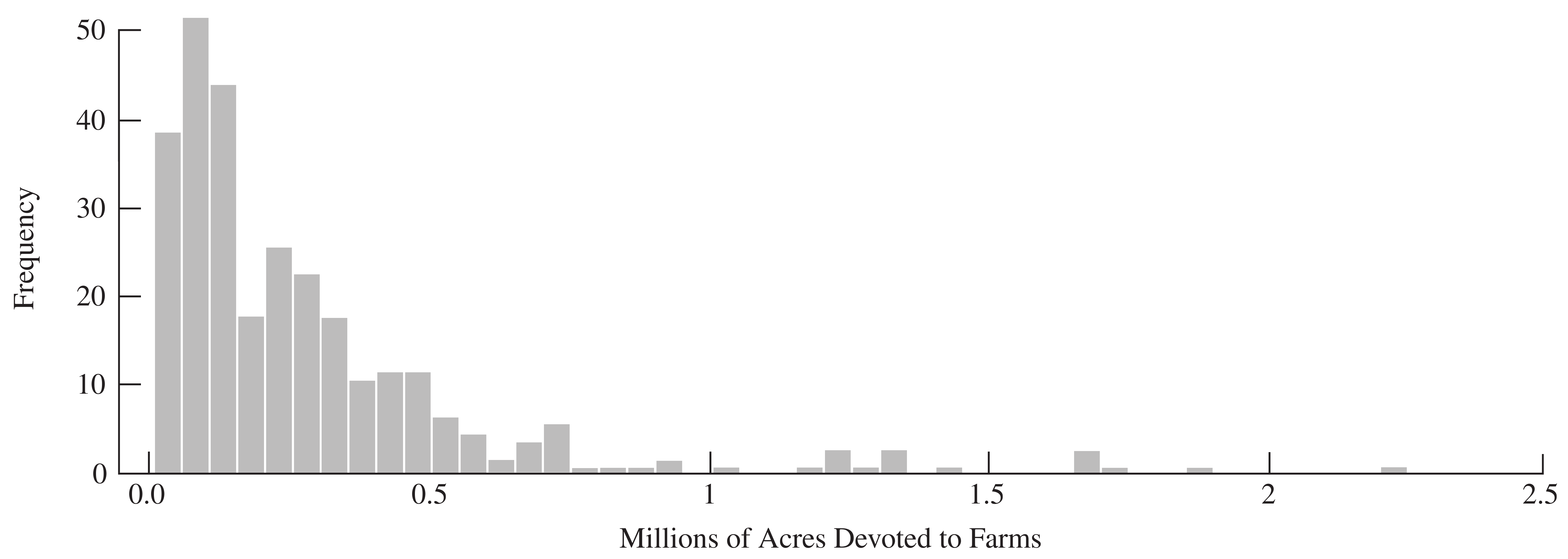
Figure 1: Histogram: number of acres devoted to farms in 1992, for an SRS of 300 counties. Note the skewness of the data. Most of the counties have fewer than 500,000 acres in farms; some counties, however, have more than 1.5 million acres in farms.

Minimum Sample Size for Normality to Hold

Sugden et al. (2000) extend Cochran’s rule for the sample size needed for the normal approximation to be adequate. A recommended minimum: n_{\min} = 28 + 25\left(\frac{\sum_{i=1}^N (y_i-\bar y_{U})^3}{N S^3}\right)^{\!2}

The quantity in parentheses is the skewness of the population; larger skewness requires a larger sample for normality to hold.

Example: Checking the Minimum Sample Size

Substituting sample values s=344{,}551.9 and \sum_{i\in\mathcal S}(y_i-\bar y)^3/n = 1.05036\times10^{17} for the corresponding population quantities: n_{\min} = 28 + 25\left(\frac{1.05036\times10^{17}}{(344{,}551.9)^3}\right)^{\!2} \approx 193

Our sample of size n=300 exceeds n_{\min}\approx193, so it appears sufficiently large for the sampling distribution of \bar y to be approximately normal.

Sample Size Estimation: Specifying Tolerable Error

The desired precision is often expressed in absolute terms: P(|\bar y - \bar y_{U}| \le e) = 1-\alpha where e is the margin of error. For many surveys of people where a proportion is measured, e=0.03 and \alpha=0.05.

Or in relative terms, controlling the CV: P\left(\left|\frac{\bar y - \bar y_{U}}{\bar y_{U}}\right| \le r\right) = 1-\alpha \quad\Longrightarrow\quad e = r \cdot \bar y_{U}

For example, if \bar y_{U}=180K and r=0.1, then e=18K.

Solving for the Required Sample Size

To obtain absolute precision e, find n satisfying e = z_{\alpha/2}\sqrt{\Big(1-\frac nN\Big)\frac{S^2}{n}}

First find the sample size n_0 we would use for an infinite population: n_0 = \left(\frac{z_{\alpha/2} S}{e}\right)^{\!2}

Then the fpc-adjusted sample size is n = \frac{n_0}{1+n_0/N} = \frac{z_{\alpha/2}^2 S^2}{e^2 + z_{\alpha/2}^2 S^2/N}

Example: Margin of Error 0.03 for a Proportion

We want to estimate the proportion of recipes in a cookbook (of N=1251 recipes) that don’t involve animal products, using a 95% CI with margin of error 0.03: n_0 = \frac{(1.96)^2 (\tfrac12)(1-\tfrac12)}{(0.03)^2} \approx 1067

Since n_0 is large relative to N=1251, we apply the fpc adjustment: n = \frac{n_0}{1+n_0/N} = \frac{1067}{1+1067/1251} = 576

If N were very large, we would use n\approx n_0 directly.

Example: Agriculture Farming Sample Size

We took a pilot sample of size 30 (one county missing acres92); the sample SD of the remaining 29 observations was 519,085. With a desired margin of error of 60,000: n_0 = (1.96)^2\,\frac{519{,}085^2}{60{,}000^2} \approx 288

With N=3078: n = \frac{n_0}{1+n_0/N} = \frac{288}{1+288/3078} \approx 263

We took a sample of size 300 in case the pilot’s estimated SD was too low.

Randomization Theory for SRS

In the randomization theory (design-based) approach, the y_i’s are considered fixed but unknown numbers; the random variables Z_i indicate which population units are in the sample: \bar y = \sum_{i\in\mathcal S} \frac{y_i}{n} = \sum_{i=1}^N Z_i \frac{y_i}{n}

The randomness in \bar y comes entirely from Z_1,\ldots,Z_N; the values y_1,\ldots,y_N are treated as fixed constants.

Distribution of Z_i

Since \{Z_1,\ldots,Z_N\} are identically distributed Bernoulli random variables with \pi_i = P(Z_i=1) = \frac{n}{N} = \frac{\binom{N-1}{n-1}}{\binom{N}{n}}, \qquad P(Z_i=0) = 1-\frac nN we get E[Z_i] = E[Z_i^2] = \frac nN V(Z_i) = E[Z_i^2] - (E[Z_i])^2 = \frac nN - \Big(\frac nN\Big)^2 = \frac nN\Big(1-\frac nN\Big)

Mean of \bar y

E[\bar y] = E\left[\sum_{i=1}^N Z_i \frac{y_i}{n}\right] = \sum_{i=1}^N E[Z_i]\frac{y_i}{n} = \sum_{i=1}^N \frac{n}{N}\cdot\frac{y_i}{n} = \sum_{i=1}^N \frac{y_i}{N} = \bar y_{U}

This shows \bar y is an unbiased estimator of \bar y_{U}.

Covariance of Z_i and Z_j

Because the population is finite, the Z_i’s are not independent: knowing unit i is in the sample gives information about unit j. For i\ne j, E[Z_iZ_j] = P(Z_j=1\mid Z_i=1)\,P(Z_i=1) = \frac{n-1}{N-1}\cdot\frac nN \text{Cov}(Z_i,Z_j) = E[Z_iZ_j]-E[Z_i]E[Z_j] = -\frac{1}{N-1}\Big(1-\frac nN\Big)\Big(\frac nN\Big)

This negative covariance is the source of the finite population correction.

Variance of \bar y

Using \text{Cov}(Z_i,Z_j) and V(Z_i), V(\bar y) = \frac{1}{n^2}\left[\sum_{i=1}^N y_i^2\, V(Z_i) + \sum_{i=1}^N\sum_{j\ne i} y_i y_j\,\text{Cov}(Z_i,Z_j)\right]

Substituting the expressions above and simplifying: V(\bar y) = \frac1n\Big(1-\frac nN\Big)\frac{1}{N(N-1)}\left[N\sum_{i=1}^N y_i^2 - \Big(\sum_{i=1}^N y_i\Big)^2\right] = \Big(1-\frac nN\Big)\frac{S^2}{n}

Proof that E(s^2) = S^2

E\left[\sum_{i\in\mathcal S}(y_i-\bar y)^2\right] = E\left[\sum_{i\in\mathcal S}(y_i-\bar y_{U})^2\right] - n\,V(\bar y) = \frac nN \sum_{i=1}^N (y_i - \bar y_{U})^2 - \Big(1-\frac nN\Big)S^2 = \frac{n(N-1)}{N}S^2 - \frac{N-n}{N}S^2 = (n-1)S^2

Therefore E\left[\frac{1}{n-1}\sum_{i\in\mathcal S}(y_i-\bar y)^2\right] = E[s^2] = S^2

STAT 348 Sampling Techniques

1 Simple Random Sampling

SRSWR and SRS

How to Do SRS?

Inclusion Probability

Estimators for the Population Mean \bar y_{U}

Variance of \bar y and Standard Error

Estimators for the Population Total t

Expression of \hat t with Sampling Weight w_i

Coefficient of Variation (CV)

Example: Census of Agriculture

Example: Estimates for acres92

Example: Calculating CV

Estimators for a Population Proportion

Variance of \hat p

Example: Proportion of Counties with Fewer than 200,000 Acres

Confidence Intervals

Normality of the Sample Mean

Confidence Intervals for SRS Estimates

Shinylive App Illustrating Central Limit Theorem

Example: CIs for agsrs.csv

Example: Skewness of Acreage Data

Minimum Sample Size for Normality to Hold

Example: Checking the Minimum Sample Size

Sample Size Estimation: Specifying Tolerable Error

Solving for the Required Sample Size

Example: Margin of Error 0.03 for a Proportion

Example: Agriculture Farming Sample Size

Randomization Theory for SRS

Distribution of Z_i

Mean of \bar y

Covariance of Z_i and Z_j

Variance of \bar y

Proof that E(s^2) = S^2

Example: Estimates for `acres92`

Example: CIs for `agsrs.csv`