STAT 348 Sampling Techniques
Stratified Random Sampling
1 What Is Stratified Sampling?
Textbook sections:
3.1–3.5 in Lohr
5.1–5.9 in Scheaffer et al.
What Is Stratified Sampling?
If the variable we are interested in takes on different mean values in different subpopulations, we may be able to obtain more precise estimates of population quantities by taking a stratified random sample. The word stratify comes from Latin words meaning “to make layers”; we divide the population into H subpopulations, called strata. The strata do not overlap, and they constitute the whole population, so that each sampling unit belongs to exactly one stratum.
We draw an independent probability sample from each stratum, then pool the information to obtain overall population estimates.
A Population Divided into Strata
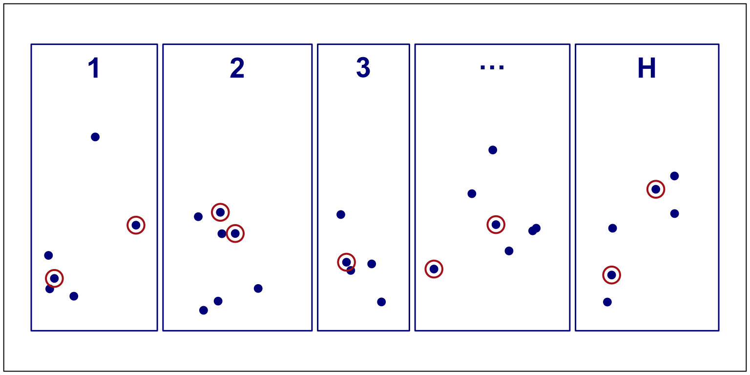
Figure 1
Each stratum h has N_h units in the population; we sample n_h of them (circled). H is the number of strata.
Example: Stratifying by Census Region
We use the four U.S. census regions as strata. The SRS in an earlier example sampled about 10% of all 3078 counties; to compare stratified sampling with SRS directly, we also sample about 10% of the counties in each stratum:
| Stratum | Counties in Stratum | Counties in Sample |
|---|---|---|
| Northeast | 220 | 21 |
| North Central | 1054 | 103 |
| South | 1382 | 135 |
| West | 422 | 41 |
| Total | 3078 | 300 |
We select four separate, independent SRSs, one per stratum. Knowing which counties are in the sample from the Northeast tells us nothing about which counties are in the sample from the South.
Example: Data Summary from Stratified Sampling
Summary statistics for acres92 in each stratum (data file agstrat.dat):
| Region (h) | Sample Size (n_h) | Average (\overline y_h) | Variance (s_h^2) |
|---|---|---|---|
| Northeast | 21 | 97,629.8 | 7,647,472,708 |
| North Central | 103 | 300,504.2 | 29,618,183,543 |
| South | 135 | 211,315.0 | 53,587,487,856 |
| West | 41 | 662,295.5 | 396,185,950,266 |
2 Estimation with Stratified Samples
Population Quantities
For unit j in stratum h, let y_{hj} denote its value, and let \pi_h = \frac{N_h}{N}, denote the proportion of population units belonging to stratum h (so \sum_{h=1}^H \pi_h = 1). Then, t_h = \sum_{j=1}^{N_h} y_{hj} \quad(\text{stratum total}) \qquad t = \sum_{h=1}^H t_h \quad(\text{population total}) \overline y_{hU} = \frac{\sum_{j=1}^{N_h} y_{hj}}{N_h} \quad(\text{stratum mean}) \qquad \overline y_U = \frac tN = \sum_{h=1}^H \pi_h\, \overline y_{hU} \quad(\text{overall mean}) S_h^2 = \frac{1}{N_h-1}\sum_{j=1}^{N_h}(y_{hj}-\overline y_{hU})^2 \quad(\text{stratum variance}).
SRS Estimators Within Each Stratum
Since an SRS is taken within each stratum, we estimate the stratum quantities using ordinary SRS formulas, applied separately to each stratum: \overline y_h = \frac{1}{n_h}\sum_{j\in\mathcal S_h} y_{hj} \qquad \hat t_h = \frac{N_h}{n_h}\sum_{j\in\mathcal S_h} y_{hj} = N_h \overline y_h s_h^2 = \sum_{j\in\mathcal S_h} \frac{(y_{hj}-\overline y_h)^2}{n_h - 1}.
Estimators for the Population Total and Mean
\hat t_{\text{str}} = \sum_{h=1}^H \hat t_h = \sum_{h=1}^H N_h \overline y_h \overline y_{\text{str}} = \frac{\hat t_{\text{str}}}{N} = \sum_{h=1}^H \pi_h\overline y_h
\overline y_{\text{str}} is a weighted average of the sample stratum averages, with \overline y_h weighted by \pi_h = N_h/N, the fraction of population units in stratum h. To use stratified sampling, the population sizes of the strata must be known.
Standard Errors for Stratified Samples
Since we sample independently across strata, variances add: V(\hat t_{\text{str}}) = \sum_{h=1}^H V(\hat t_h) = \sum_{h=1}^H \Big(1-\frac{n_h}{N_h}\Big)N_h^2\frac{S_h^2}{n_h}.
Substituting sample variances s_h^2 for S_h^2 gives unbiased estimators: \hat V(\hat t_{\text{str}}) = \sum_{h=1}^H \Big(1-\frac{n_h}{N_h}\Big)N_h^2\frac{s_h^2}{n_h} \hat V(\overline y_{\text{str}}) = \frac{1}{N^2}\hat V(\hat t_{\text{str}}) = \sum_{h=1}^H \Big(1-\frac{n_h}{N_h}\Big)\pi_h^2\frac{s_h^2}{n_h}.
Note we need at least two sampled units per stratum to estimate the variances.
Unbiasedness of \overline y_{\text{str}}
E\left[\sum_{h=1}^H \frac{N_h}{N}\overline y_h\right] = \sum_{h=1}^H \frac{N_h}{N}E[\overline y_h] = \sum_{h=1}^H \frac{N_h}{N}\overline y_{hU} = \sum_{h=1}^H \frac{N_h}{N}\cdot \frac{\sum_{j=1}^{N_h} y_{hj}}{N_h} = \sum_{h=1}^H \frac{\sum_{j=1}^{N_h}y_{hj}}{N} = \overline y_U.
Since an SRS is taken in each stratum, E[\overline y_h]=\overline y_{hU}; averaging these unbiased stratum estimates with weights N_h/N keeps the overall estimate unbiased.
Confidence Intervals for Stratified Samples
If either (1) the sample sizes within each stratum are large, or (2) the sampling design has a large number of strata, an approximate 100(1-\alpha)\% CI for \overline y_U is \overline y_{\text{str}} \pm z_{\alpha/2}\,\text{SE}(\overline y_{\text{str}}).
When n is not large, it is common to use the quantile of a t distribution with n-H degrees of freedom instead of the normal quantile: \hat t_{\text{str}} \pm t_{\alpha/2,\,n-H}\cdot \text{SE}(\hat t_{\text{str}}).
Example 1: The Nelchina Caribou Herd
Siniff and Skoog (1964) used stratified random sampling to estimate the size of the Nelchina herd of Alaska caribou in February 1962. Preliminary caribou density estimates were used to divide the area of interest into six strata; each stratum was divided into a grid of 4-mi^2 sampling units. Stratum A, for example, contained N_1=400 sampling units, of which n_1=98 were randomly selected for the survey.
Example 1: Strata Layout
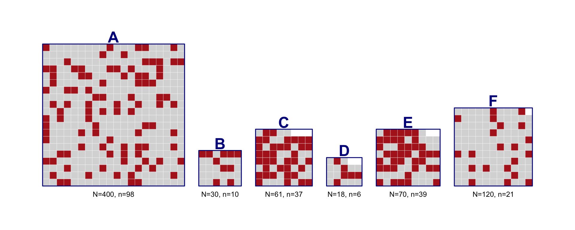
Figure 2
Each grid represents one stratum’s N_h sampling units; the highlighted (red) cells are the n_h units randomly selected in that stratum.
Example 1: Spreadsheet for Calculations
Here \pi_h = N_h/N with N=699, and the last two columns give each stratum’s contribution to \overline y_{\text{str}}=\sum_h \pi_h\overline y_h and to \hat V(\overline y_{\text{str}}) = \sum_h\big(1-\tfrac{n_h}{N_h}\big)\pi_h^2\tfrac{s_h^2}{n_h}:
| Stratum | N_h | n_h | \pi_h=N_h/N | \overline y_h | s_h^2 | \pi_h\overline y_h | \hat v_h1 |
|---|---|---|---|---|---|---|---|
| A | 400 | 98 | 0.5722 | 24.1 | 5,575 | 13.7911 | 14.0648 |
| B | 30 | 10 | 0.0429 | 25.6 | 4,064 | 1.0987 | 0.4991 |
| C | 61 | 37 | 0.0873 | 267.6 | 347,556 | 23.3528 | 28.1455 |
| D | 18 | 6 | 0.0258 | 179.0 | 22,798 | 4.6094 | 1.6798 |
| E | 70 | 39 | 0.1001 | 293.7 | 123,578 | 29.4120 | 14.0728 |
| F | 120 | 21 | 0.1717 | 33.2 | 9,795 | 5.6996 | 11.3409 |
| Total | 699 | 211 | 1.0000 | 77.9636 | 69.8029 |
Example 1: Results
The estimated mean number of caribou per sampling unit is \overline y_{\text{str}} = 77.96, \text{SE}(\overline y_{\text{str}}) = \sqrt{69.8029} = 8.35.
The estimated total number of caribou: \hat t_{\text{str}} = N\overline y_{\text{str}} = 699(77.96) = 54{,}497, \text{SE}(\hat t_{\text{str}}) = N\cdot\text{SE}(\overline y_{\text{str}}) = 699(8.35) = 5{,}840.
An approximate 95% CI for the total number of caribou: 54{,}497 \pm 1.96(5840) = [43{,}051,\ 65{,}943].
This CI reflects only sampling error; if the field procedure for counting caribou tends to miss animals, the entire CI will be biased low.
Example 2: Estimated Farm Acreage by Region
Using the same census-region strata for acres92:
| Stratum | Estimated Total of Farm Acres | Estimated Variance of Total |
|---|---|---|
| Northeast | 21,478,558.2 | 1.5943\times10^{13} |
| North Central | 316,731,379.4 | 2.8823\times10^{14} |
| South | 292,037,390.8 | 6.8408\times10^{14} |
| West | 279,488,706.1 | 1.5537\times10^{15} |
| Total | 909,736,034.4 | 2.5419\times10^{15} |
Since sampling was independent across strata, the variance of the U.S. total is the sum of the four stratum variances.
Example 2: Results
\hat t_{\text{str}} = 909{,}736{,}034, \qquad \text{SE}(\hat t_{\text{str}}) = \sqrt{2.5419\times10^{15}} = 50{,}417{,}248.
The average number of acres devoted to farming per county: \overline y_{\text{str}} = \frac{909{,}736{,}034}{3078} = 295{,}560.76, \qquad \text{SE}(\overline y_{\text{str}}) = \frac{50{,}417{,}248}{3078} = 16{,}379.87.
Comparison of Stratified Sampling and SRS
Only the West had sample variance larger than the overall SRS sample variance; the sample variance in the Northeast was much smaller than the population as a whole. Observations within many strata tend to be more homogeneous than observations in the population overall.
The relative gain from stratification can be estimated by the ratio \frac{\text{estimated variance from stratified sample},\ n=300}{\text{estimated variance from SRS},\ n=300} = \frac{2.5419\times10^{15}}{3.3837\times10^{15}} = 0.75.
Percentage of variance reduction = 1-0.75 = 0.25. If these were the population variances, we would need only (300)(0.75)=225 observations with a stratified sample to match the precision of an SRS of 300.
3 Stratified Sampling for Proportions
Estimators for a Population Proportion p
A proportion is the mean of a 0/1 variable, so we apply the same formulas with \overline y_h = \hat p_h and s_h^2 = \frac{n_h}{n_h-1}\hat p_h(1-\hat p_h): \hat p_{\text{str}} = \sum_{h=1}^H \frac{N_h}{N}\hat p_h \hat V(\hat p_{\text{str}}) = \sum_{h=1}^H \Big(1-\frac{n_h}{N_h}\Big)\Big(\frac{N_h}{N}\Big)^2\frac{\hat p_h(1-\hat p_h)}{n_h-1}.
Example: ACLS Survey of Scholars
The American Council of Learned Societies (ACLS) used a stratified random sample of member societies in seven disciplines to study publication patterns and computer/library use (Morton and Price, 1989).
| Discipline | Membership (N_h) | Valid Returns (n_h) | Female Members (%) |
|---|---|---|---|
| Literature | 9,100 | 636 | 38 |
| Classics | 1,950 | 451 | 27 |
| Philosophy | 5,500 | 481 | 18 |
| History | 10,850 | 611 | 19 |
| Linguistics | 2,100 | 493 | 36 |
| Political Science | 5,500 | 575 | 13 |
| Sociology | 9,000 | 588 | 26 |
| Totals | 44,000 | 3,835 |
Example: ACLS Spreadsheet Calculation
Here \pi_h = N_h/N with N=44{,}000, and the last two columns give each stratum’s contribution to \hat p_{\text{str}}=\sum_h \pi_h\hat p_h and to \hat V(\hat p_{\text{str}})=\sum_h\big(1-\tfrac{n_h}{N_h}\big)\pi_h^2\tfrac{\hat p_h(1-\hat p_h)}{n_h-1}:
| Discipline | N_h | n_h | \pi_h=N_h/N | \hat p_h | \pi_h\hat p_h | \hat v_h (\times10^{-5})1 |
|---|---|---|---|---|---|---|
| Literature | 9,100 | 636 | 0.2068 | 0.38 | 0.0786 | 1.476 |
| Classics | 1,950 | 451 | 0.0443 | 0.27 | 0.0120 | 0.066 |
| Philosophy | 5,500 | 481 | 0.1250 | 0.18 | 0.0225 | 0.439 |
| History | 10,850 | 611 | 0.2466 | 0.19 | 0.0469 | 1.448 |
| Linguistics | 2,100 | 493 | 0.0477 | 0.36 | 0.0172 | 0.082 |
| Political Science | 5,500 | 575 | 0.1250 | 0.13 | 0.0163 | 0.276 |
| Sociology | 9,000 | 588 | 0.2045 | 0.26 | 0.0532 | 1.282 |
| Total | 44,000 | 3,835 | 1.0000 | 0.2465 | 5.068 |
Example: ACLS Estimates
Let N_h be the membership figures and n_h the number of valid surveys. Ignoring nonresponse for now, and estimating the proportion of these scholars who are female: \hat p_{\text{str}} = \sum_{h=1}^7 \frac{N_h}{N}\hat p_h = \frac{9100}{44{,}000}(0.38) + \cdots + \frac{9000}{44{,}000}(0.26) = 0.2465 \text{SE}(\hat p_{\text{str}}) = \sqrt{\sum_{h=1}^7 \Big(1-\frac{n_h}{N_h}\Big)\Big(\frac{N_h}{N}\Big)^2\frac{\hat p_h(1-\hat p_h)}{n_h-1}} = 0.0071.
To estimate the total number of female scholars, multiply N=44{,}000 by these two numbers.
4 Comparison with SRS Formulas
In contrast, if we had taken an SRS of size n=n_1+\cdots+n_H from the whole population, the sample mean would be \overline y_{\text{SRS}} = \frac{\sum_{(h,j)\in\mathcal S} y_{hj}}{n} = \frac{\overline y_1 n_1 + \cdots + \overline y_H n_H}{n} = \overline y_1\frac{n_1}{n} + \cdots + \overline y_H\frac{n_H}{n},
compared with the stratified estimator \overline y_{\text{str}} = \overline y_1\frac{N_1}{N} + \cdots + \overline y_H\frac{N_H}{N}.
Comparison with SRS Formulas (cont’d)
Similarly, for proportions: \hat p_{\text{SRS}} = \sum_{h=1}^H \frac{n_h}{n}\hat p_h = \sum_{h=1}^H \frac{n_h \hat p_h}{n}.
The key difference: \overline y_{\text{SRS}} weights each stratum’s sample mean by its realized sample fraction n_h/n, which may be influenced by sampling variation and by non-response rates. \overline y_{\text{str}} instead uses the known, fixed population fraction N_h/N for each stratum, which is what guarantees unbiasedness for \overline y_U.
5 Sampling Weights for Stratified Sampling
Sampling Probabilities for Each Sample
Write the overall stratified sample as \mathcal S = (\mathcal S_1,\ldots,\mathcal S_H), where \mathcal S_h is the SRS drawn from stratum h. Since the strata are sampled independently, P(\mathcal S) = P(\mathcal S_1)\times P(\mathcal S_2)\times\cdots\times P(\mathcal S_H) = \frac{1}{\binom{N_1}{n_1}}\cdot\frac{1}{\binom{N_2}{n_2}}\cdots\frac{1}{\binom{N_H}{n_H}}.
Sampling Weights
We introduced the sampling weight w_i = 1/\pi_i for SRS. For unit j in stratum h, the inclusion probability is \pi_{hj} = n_h/N_h (the sampling fraction in stratum h), so the sampling weight is, w_{hj} = \frac{1}{\pi_{hj}} = \frac{N_h}{n_h}.
Stratified sampling is an example of unequal-probability sampling.
The sampling weight can be thought of as the number of population units represented by the sampled unit. Within stratum h, all n_h sampled units have the same weight N_h/n_h, so \sum_{j\in\mathcal S_h} w_{hj} = n_h\cdot\frac{N_h}{n_h} = N_h, \qquad \sum_{h=1}^H\sum_{j\in\mathcal S_h} w_{hj} = \sum_{h=1}^H N_h = N.
Estimators in Terms of Sampling Weights
Since N_h\overline y_h = \dfrac{N_h}{n_h}\displaystyle\sum_{j\in\mathcal S_h} y_{hj} = \sum_{j\in\mathcal S_h} w_{hj}\,y_{hj}, the population total can be written as a weighted sum over all sampled units, regardless of stratum: \hat t_{\text{str}} = \sum_{h=1}^H N_h \overline y_h = \sum_{h=1}^H \sum_{j\in\mathcal S_h} w_{hj}\, y_{hj}.
Since the weights sum to N, the population mean can also be written \overline y_{\text{str}} = \frac{\hat t_{\text{str}}}{N} = \frac{\displaystyle\sum_{h=1}^H\sum_{j\in\mathcal S_h} w_{hj}y_{hj}}{\displaystyle\sum_{h=1}^H\sum_{j\in\mathcal S_h} w_{hj}}.
Example: Weights for the Caribou Survey
| Stratum | N_h | n_h | w_{hj} = N_h/n_h |
|---|---|---|---|
| A | 400 | 98 | 4.08 |
| B | 30 | 10 | 3.00 |
| C | 61 | 37 | 1.65 |
| D | 18 | 6 | 3.00 |
| E | 70 | 39 | 1.79 |
| F | 120 | 21 | 5.71 |
Note that using only the weights w_{hj} and sample sizes n_h is not enough to estimate variances — that requires computing s_h^2 separately within each stratum, since the weights alone don’t identify stratum membership.
6 Efficiency of Proportional Allocation
Proportional Allocation
A special case, useful for comparing with SRS: proportional allocation takes the same sampling fraction in every stratum, \frac{n_h}{N_h} = \frac nN \quad \text{for all } h.
This is not an optimal allocation in general, but it is a convenient benchmark.
Decomposition of Population Variance
| Source | df | Sum of Squares |
|---|---|---|
| Between strata | H-1 | \text{SSB} = \sum_{h=1}^H N_h(\overline y_{hU}-\overline y_U)^2 |
| Within strata | N-H | \text{SSW} = \sum_{h=1}^H (N_h-1)S_h^2 |
| Total, about \overline y_U | N-1 | \text{SSTO} = (N-1)S^2 |
\text{SSTO} = \text{SSB} + \text{SSW}.
Sum Squares of Prediction Errors
Define two prediction vectors for y as follows: \begin{array}{c|ccc|c|ccc} & & \text{stratum } 1 & & \cdots & & \text{stratum } H & \\ \hline \boldsymbol y^\top & y_{11} & \cdots & y_{1N_1} & \cdots & y_{H1} & \cdots & y_{HN_H}\\ \hat{\boldsymbol y}_0^\top & \overline y_U & \cdots & \overline y_U & \cdots & \overline y_U & \cdots & \overline y_U\\ \hat{\boldsymbol y}_1^\top & \overline y_{1U} & \cdots & \overline y_{1U} & \cdots & \overline y_{HU} & \cdots & \overline y_{HU} \end{array}
\hat{\boldsymbol y}_0 ignores the strata; \hat{\boldsymbol y}_1 predicts each unit by its stratum mean. Then \text{SSTO} = \|\boldsymbol y-\hat{\boldsymbol y}_0\|^2,\qquad \text{SSW} = \|\boldsymbol y-\hat{\boldsymbol y}_1\|^2, \text{SSB} = \|\hat{\boldsymbol y}_1-\hat{\boldsymbol y}_0\|^2 = \sum_{h=1}^H N_h(\overline y_{hU}-\overline y_U)^2.
Since \boldsymbol y-\hat{\boldsymbol y}_0 = (\boldsymbol y-\hat{\boldsymbol y}_1) + (\hat{\boldsymbol y}_1-\hat{\boldsymbol y}_0) and the two pieces are orthogonal, \text{SSTO} = \text{SSW} + \text{SSB}.
Illustration of SSB and SSW
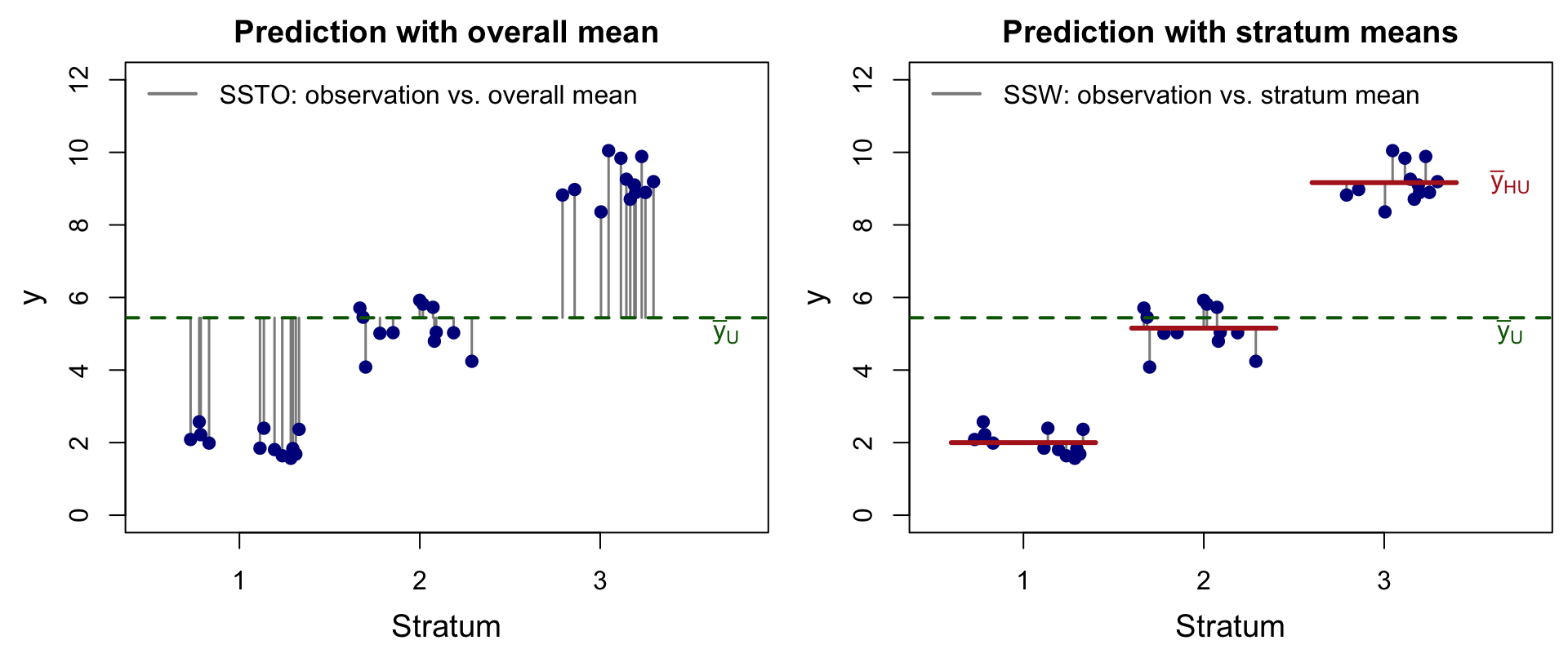
Figure 3
Left: predicting every observation by the overall mean (green dashed line); the squared errors (grey) sum to SSTO. Right: predicting each observation by its stratum mean (red segments); the squared errors (grey) sum to SSW. The difference SSTO - SSW is SSB, the sum of squared distances from each observation’s stratum mean to the overall mean.
Coefficient of Determination R^2
R^2 = 1-\frac{\text{SSW}}{\text{SST}} = \frac{\text{SSB}}{\text{SST}}
R^2 generalizes the squared Pearson correlation coefficient: it measures the correlation between a response y and one or more predictors x_1,\ldots,x_p — here, “stratum membership” plays the role of the predictor. R^2 is the proportion of the variance in y explained by the predictors.
R^2 Large vs. R^2 Small
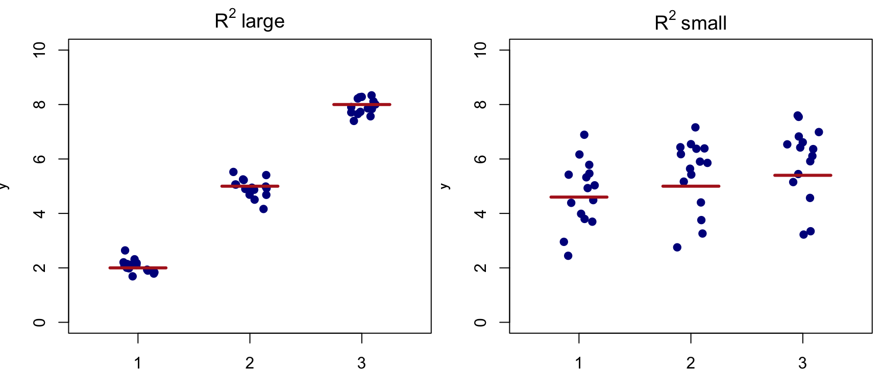
Figure 4
When the strata means differ widely relative to the within-stratum spread (left), stratification explains a large share of the variance in y.
Comparing Variances: Proportional Allocation vs. SRS
For a stratified sample of size n with proportional allocation, V_{\text{prop}}(\hat t_{\text{str}}) = \sum_{h=1}^H \Big(1-\frac nN\Big)\frac Nn\, N_h S_h^2 = \Big(1-\frac nN\Big)\frac Nn\left(\text{SSW} + \sum_{h=1}^H S_h^2\right).
Since \text{SSTO}=\text{SSW}+\text{SSB}, the variance of the total from an SRS of size n is. V_{\text{SRS}}(\hat t) = \Big(1-\frac nN\Big)\frac{N^2 S^2}{n} = \Big(1-\frac nN\Big)\frac{N^2}{n(N-1)}(\text{SSW}+\text{SSB}).
When Does Stratification Help?
Comparing the two expressions, proportional allocation gives smaller variance than SRS whenever \text{SSB} > \sum_{h=1}^H \Big(1-\frac{N_h}{N}\Big)S_h^2.
This typically holds because SSB is a sum of N squared deviations, while \sum_h S_h^2 is a sum of only H (typically much fewer) terms.
The Variance Ratio and R^2
\frac{V_{\text{prop}}(\hat t_{\text{str}})}{V(\hat t_{\text{SRS}})} \approx \frac{\text{SSW}+\sum_h S_h^2}{\text{SSW}+\text{SSB}} \approx \frac{\text{SSW}}{\text{SSW}+\text{SSB}} \text{percentage of variance reduction} = \frac{\text{SSB}}{\text{SSW}+\text{SSB}} = R^2_{y\mid\text{strata}},
the proportion of variance in y that can be explained by strata membership.
7 Optimal Allocation
Setting Up the Cost Function
The objective in optimal allocation is to gain the most information for the least cost. Let C be total cost, c_0 overhead cost, and c_h the cost of sampling one unit in stratum h: C = c_0 + \sum_{h=1}^H c_h n_h, \qquad n = n_1+\cdots+n_H.
We want to allocate n_1,\ldots,n_H to minimize V(\overline y_{\text{str}}) for a fixed total cost C (or equivalently minimize C for fixed V).
Deriving the Optimal Allocation
Write the variance as V(\overline y_{\text{str}}) = \sum_{h=1}^H \Big(1-\frac{n_h}{N_h}\Big)\frac{N_h^2}{N^2}\frac{S_h^2}{n_h} = \sum_{h=1}^H \frac{N_h^2S_h^2}{N^2}\cdot\frac1{n_h} \;-\; \underbrace{\sum_{h=1}^H \frac{N_hS_h^2}{N^2}}_{\text{free of } n_h}.
Minimize it subject to c_0+\sum_h c_hn_h = C using the Lagrangian L(n_1,\ldots,n_H,\lambda) = \sum_{h=1}^H \frac{N_h^2S_h^2}{N^2 n_h} + \lambda\Big(c_0+\sum_{h=1}^H c_hn_h - C\Big).
Setting \partial L/\partial n_h = 0: -\frac{N_h^2S_h^2}{N^2n_h^2} + \lambda c_h = 0 \quad\Longrightarrow\quad n_h = \frac{1}{N\sqrt\lambda}\cdot\frac{N_hS_h}{\sqrt{c_h}} \;\propto\; \frac{N_hS_h}{\sqrt{c_h}}.
Summing over h gives n = \frac{1}{N\sqrt\lambda}\sum_{l} N_lS_l/\sqrt{c_l}; dividing n_h by n eliminates \lambda and yields the formula on the next slide.
Optimal Allocation Formula
Using the method of Lagrange multipliers, the optimal n_h is proportional to N_hS_h/\sqrt{c_h}: n_h = \left(\frac{N_hS_h/\sqrt{c_h}}{\sum_{l=1}^H N_lS_l/\sqrt{c_l}}\right)n \qquad\text{i.e.}\qquad n_h \propto \frac{N_hS_h}{\sqrt{c_h}}.
We sample more heavily within a stratum if: the stratum is a large part of the population (N_h large); the stratum is more variable (S_h large); or sampling in the stratum is cheap (c_h small).
Special cases: if c_1=\cdots=c_H, then n_h\propto N_hS_h (Neyman allocation); if additionally S_1=\cdots=S_H, then n_h\propto N_h (proportional allocation).
Example: Neyman Allocation for the Caribou Survey
The investigators used rough estimates of caribou counts as a proxy for S_h, with total sample size n=225:
| Stratum | N_h | s_h | N_hs_h | n_h (Neyman) | Sample size used |
|---|---|---|---|---|---|
| A | 400 | 3,000 | 1,200,000 | 96.26 | 98 |
| B | 30 | 2,000 | 60,000 | 4.81 | 10 |
| C | 61 | 9,000 | 549,000 | 44.04 | 37 |
| D | 18 | 2,000 | 36,000 | 2.89 | 6 |
| E | 70 | 12,000 | 840,000 | 67.38 | 39 |
| F | 120 | 1,000 | 120,000 | 9.63 | 21 |
| Total | 699 | 2,805,000 | 225 | 211 |
They wanted the sampling fraction to be at least 1/3 in the smaller strata, so the Neyman values (column n_h) were used only as a guideline.
Example: Optimal Allocation for Polls
For estimating a proportion, S_h^2 = p_h(1-p_h). As a function of p, S^2(p)=p(1-p) is a quadratic maximized at p=1/2. So election regions (swing states) with p near 0.5 should be assigned relatively larger sample sizes, since they contribute the most variance per unit sampled.
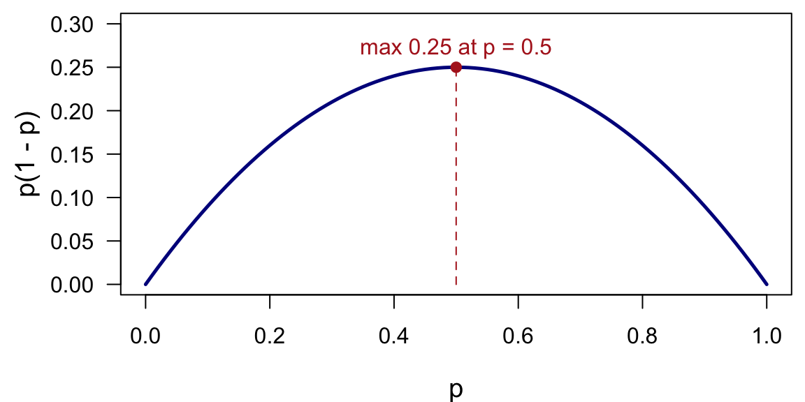
Figure 5
Example: Dollar Stratification
Dollar stratification is common in accounting audits. Recorded book amounts stratify the population: stratum 1 might be all loans over $1 million, stratum 2 loans between $500,000 and $999,999, and so on down to loans under $10,000.
Optimal allocation is efficient here: S_h is much larger in strata with large loan amounts, so optimal allocation prescribes a higher sampling fraction for those strata. An error in a $3,000,000 loan is likely to contribute far more to the total audited discrepancy than an error in a $3,000 loan.
8 Choice of Stratifying Variables
Using an Auxiliary Variable
Stratification is most efficient when the stratum means differ widely, since then SSB is large and within-stratum variability is small. Ideally we would stratify directly by the values of y; since y is unknown before sampling, we instead look for an auxiliary variable x that is highly correlated with (or predictive of) y.
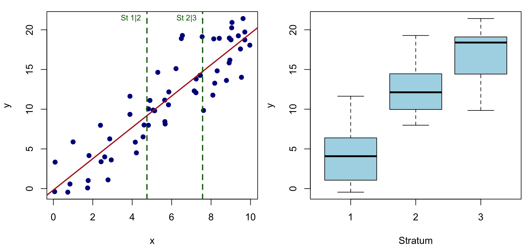
Figure 6
Cutting on x (left) produces strata with visibly different distributions of y (right) — exactly the goal of stratification.
Example: Choosing an Auxiliary Variable
To estimate total business expenditures on advertising, we would like businesses that spend the most on advertising in stratum 1, the next highest spenders in stratum 2, and so on. We might stratify by number of employees or size of business, and by type of product or service.
For farm income, we might use farm size as the stratifying variable, since we expect larger farms to have higher incomes.
Limitations of Stratified Sampling
Difficulty in implementation. We need to know the stratum sizes N_h (and, for optimal allocation, rough estimates of S_h) before sampling.
Multiple variables of interest. A single stratifying variable that works well for one y may not work well for another y measured in the same survey — a variable highly correlated with one outcome may be nearly uncorrelated with a different outcome of interest.