STAT 348 Sampling Techniques
Cluster Sampling
1 General Terms for Cluster Sampling
Textbook sections:
- 5.1–5.3 in Lohr
- Ch 8 and 9 in Scheaffer et al.
An Example of Clusters
Suppose we want to find out how many bicycles are owned by residents in a community of 10,000 households. We could take an SRS of 400 households, or we could divide the community into blocks of about 20 households each and sample every household (or subsample some households) in each of 20 blocks selected at random from the 500 blocks in the community.
The latter plan is an example of cluster sampling. The blocks are the primary sampling units (psus), or clusters. The households are the secondary sampling units (ssus); often the ssus are the elements of the population.
Why Do We Use Cluster Sampling?
- Constructing a sampling frame of observation units may be difficult, expensive, or impossible. We cannot list all honeybees in a region or all customers of a store; we may be able to construct a list of individuals in a city only via a list of housing units, but that list is time-consuming and expensive to build.
- The population may be widely spread out geographically, or occur in natural clusters such as households or schools, and it is cheaper to sample clusters than to take an SRS of individuals. To survey nursing-home residents, it is much cheaper to sample nursing homes and interview every resident there than to take an SRS of residents (which might require traveling to a home to interview just one person).
Cluster Sampling vs. Stratified Sampling
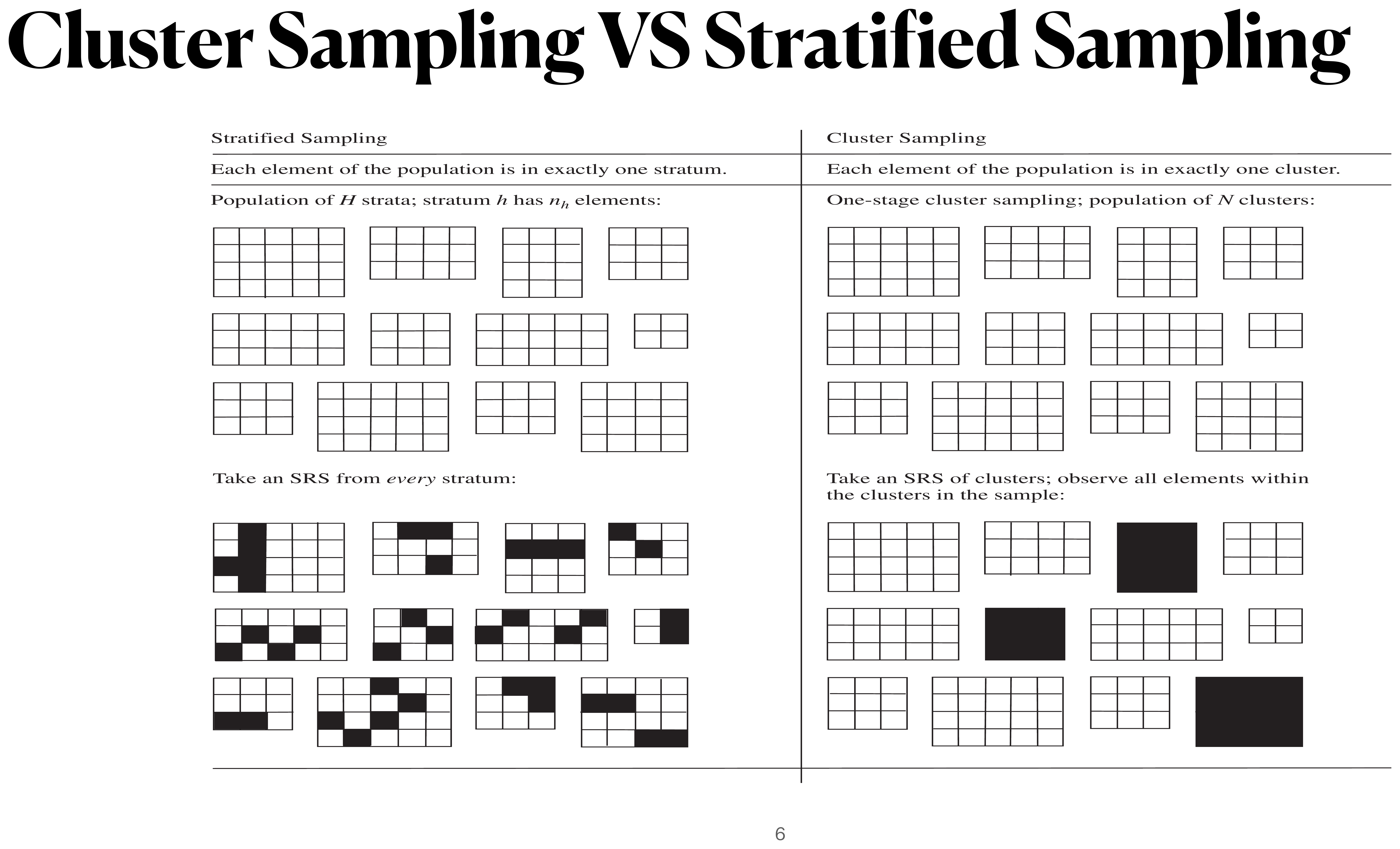
In stratified sampling, every stratum is sampled and precision depends on within-stratum homogeneity. In cluster sampling, only some clusters are sampled and precision depends primarily on the variability between cluster means.
Notation for Cluster Sampling
The universe \mathcal U is the population of N psus; \mathcal S is the sample of psus, and \mathcal S_i is the sample of ssus chosen from psu i. The measured quantity is y_{ij} = \text{measurement for the } j\text{th element (ssu) in the } i\text{th psu.}
In cluster sampling, N is the number of psus, not the number of observation units — a departure from earlier chapters where N was the population size in elements.
psu-Level Population Quantities
N = \text{number of psus}, \qquad M_i = \text{number of ssus in psu } i, \qquad M_0 = \sum_{i=1}^N M_i t_i = \sum_{j=1}^{M_i} y_{ij} \quad(\text{psu total}) \qquad t = \sum_{i=1}^N t_i \quad(\text{population total}) S_t^2 = \frac{1}{N-1}\sum_{i=1}^N \Big(t_i - \frac tN\Big)^2 \quad(\text{population variance of psu totals})
ssu-Level Population Quantities
\bar y_U = \frac{\sum_{i=1}^N\sum_{j=1}^{M_i} y_{ij}}{M_0} = \frac{t}{M_0} \quad(\text{population mean}) \bar y_{iU} = \frac{\sum_{j=1}^{M_i} y_{ij}}{M_i} = \frac{t_i}{M_i} \quad(\text{population mean in psu } i) S^2 = \frac{\sum_{i=1}^N\sum_{j=1}^{M_i}(y_{ij}-\bar y_U)^2}{M_0-1} \quad(\text{population variance}) S_i^2 = \frac{\sum_{j=1}^{M_i}(y_{ij}-\bar y_{iU})^2}{M_i-1} \quad(\text{population variance within psu } i)
Sample Quantities
Let n = number of psus sampled, m_i = number of ssus sampled from psu i: \bar y_i = \frac{\sum_{j\in\mathcal S_i} y_{ij}}{m_i} \quad\qquad \hat t_i = \sum_{j\in\mathcal S_i} \frac{M_i}{m_i}y_{ij} = M_i\bar y_i \hat t_{\text{unb}} = \sum_{i\in\mathcal S} \frac{N}{n}\hat t_i \quad(\text{unbiased estimator of } t) \bar t = \frac{\sum_{i\in\mathcal S} \hat t_i}{n}, \qquad s_t^2 = \frac{1}{n-1}\sum_{i\in\mathcal S} \big(\hat t_i - \bar t\big)^2
Sampling Weights
The probability that ssu j in psu i is selected: \begin{aligned} P(j\text{th ssu of }i\text{th psu selected}) &= P(i\text{th psu selected})\times P(j\text{th ssu}\mid i\text{th psu}) \\[4pt] &= \frac nN \cdot \frac{m_i}{M_i} \end{aligned}
So the sampling weight (reciprocal of the selection probability) is w_{ij} = \frac{N}{n}\cdot\frac{M_i}{m_i}, \qquad \hat t_{\text{unb}} = \sum_{i\in\mathcal S}\sum_{j\in\mathcal S_i} w_{ij}y_{ij}
If psus are blocks and ssus are households, household j in psu i represents (NM_i)/(nm_i) households in the population.
2 One-Stage Cluster Sampling
Clusters of Equal Sizes
Consider the simplest case, where every psu has the same number of ssus, M_i=m_i=M (all ssus sampled, all clusters same size). This is uncommon in household surveys but does occur in agricultural and industrial sampling.
Since we observe every ssu in each sampled psu, estimating population means or totals is simple: we treat the psu totals t_i as the observations and ignore the individual elements — we effectively have an SRS of n data points \{t_i, i\in\mathcal S\}.
Estimators for Clusters of Equal Sizes
Apply ordinary SRS results to the psu totals \{t_i\}: \bar t = \frac{\sum_{i\in\mathcal S} t_i}{n}, \qquad \hat t = N\bar t, \qquad s_t^2 = \frac{1}{n-1}\sum_{i\in\mathcal S}\Big(t_i-\frac{\hat t}{N}\Big)^2 \text{SE}(\hat t) = N\sqrt{\Big(1-\frac nN\Big)\frac{s_t^2}{n}}
To estimate \bar y_U, divide the estimated total by the number of elements NM: \hat{\bar y} = \frac{\hat t}{NM}, \qquad \text{SE}(\hat{\bar y}) = \frac{1}{M}\sqrt{\Big(1-\frac nN\Big)\frac{s_t^2}{n}} = \frac{\text{SE}(\bar t)}{M}
Example: GPA in a Dormitory
A student wants to estimate the average GPA in his dormitory. Instead of listing all students and taking an SRS, he notices the dorm consists of 100 suites of 4 students each; he selects 5 suites at random and asks every person in those suites for their GPA:
| Suite | Person 1 | Person 2 | Person 3 | Person 4 | Total (t_i) |
|---|---|---|---|---|---|
| 1 | 3.08 | 2.60 | 3.44 | 3.04 | 12.16 |
| 2 | 2.36 | 3.04 | 3.28 | 2.68 | 11.36 |
| 3 | 2.00 | 2.56 | 2.52 | 1.88 | 8.96 |
| 4 | 3.00 | 2.88 | 3.44 | 3.64 | 12.96 |
| 5 | 2.68 | 1.92 | 3.28 | 3.20 | 11.08 |
The psus are the suites: N=100, n=5, M=4.
Example: GPA Calculations
\begin{aligned} \hat t &= \frac{100}{5}(12.16+11.36+8.96+12.96+11.08) = 1130.4 \\[4pt] \bar t &= \frac{1130.4}{100} = 11.304 \\[4pt] s_t^2 &= \frac{1}{4}\Big[(12.16-11.304)^2+\cdots+(11.08-11.304)^2\Big] = 2.256 \\[4pt] \hat{\bar y} &= \frac{1130.4}{400} = 2.826 \\[4pt] \text{SE}(\hat{\bar y}) &= \sqrt{\Big(1-\frac{5}{100}\Big)\frac{2.256}{(5)(4)^2}} = 0.164 \end{aligned}
Note
V(\hat{\bar y}) \ne \big(1-\tfrac{n}{N}\big)\dfrac{s_y^2}{n}! We cannot apply the ordinary one-stage SRS variance formula treating all nM=20 students as an SRS from the dorm — the 20 students are not an SRS of individuals, since whole suites are selected together (an ICC/correlation effect).
3 Comparing Cluster Sampling with SRS
Population ANOVA Table (Cluster Sampling, Equal Sizes)
| Source | df | Sum of Squares |
|---|---|---|
| Between psus | N-1 | \text{SSB} = \sum_{i=1}^N\sum_{j=1}^M (\bar y_{iU}-\bar y_U)^2 |
| Within psus | N(M-1) | \text{SSW} = \sum_{i=1}^N\sum_{j=1}^M (y_{ij}-\bar y_{iU})^2 |
| Total, about \bar y_U | NM-1 | \text{SSTO} = \sum_{i=1}^N\sum_{j=1}^M (y_{ij}-\bar y_U)^2 = (NM-1)S^2 |
Cluster Sampling Variance Depends on Between-psu Variability
Since each psu has the same size M, S_t^2 = \sum_{i=1}^N \frac{(t_i-\bar t_U)^2}{N-1} = \sum_{i=1}^N \frac{M^2(\bar y_{iU}-\bar y_U)^2}{N-1} = M(\text{MSB}) so for one-stage cluster sampling with equal-size clusters, V(\hat t_{\text{cluster}}) = N^2\Big(1-\frac nN\Big)\frac{M(\text{MSB})}{n}
If instead we took an SRS with nM observations, the variance of the estimated total would have been V(\hat t_{\text{SRS}}) = (NM)^2\Big(1-\frac{nM}{NM}\Big)\frac{S^2}{nM} = N^2\Big(1-\frac nN\Big)\frac{MS^2}{n}
Comparing the two: if \text{MSB} > S^2, cluster sampling is less efficient (has larger variance) than an SRS of the same number of elements.
Intraclass Correlation and Adjusted R^2
The intraclass correlation coefficient (ICC) measures how similar elements within the same cluster are: \text{ICC} = 1 - \frac{M}{M-1}\cdot\frac{\text{SSW}}{\text{SSTO}}
An alternative measure, valid for unequal cluster sizes too, is the adjusted R^2: R_a^2 = 1 - \frac{\text{MSW}}{S^2}
For equal-sized clusters, the increase in variance from using cluster sampling (instead of an SRS of the same number of elements) is \frac{V(\hat t_{\text{cluster}})}{V(\hat t_{\text{SRS}})} = \frac{\text{MSB}}{S^2} = 1 + \frac{N(M-1)}{N-1}R_a^2
So (M-1)R_a^2 is (approximately) the percentage increase in variance from switching from SRS to cluster sampling.
Illustration: R_a^2 Large vs. Small
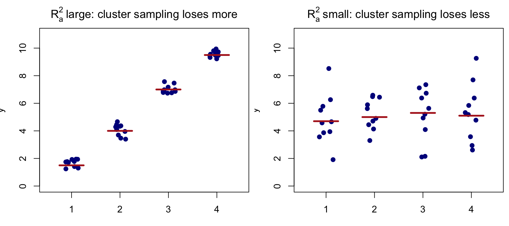
Figure 1
When cluster means differ a lot relative to within-cluster spread (left), sampling only a few clusters misses most of the population’s variability — cluster sampling loses more information relative to an SRS of the same size.
4 Clusters of Unequal Sizes
Unbiased Estimation for Unequal-Size Clusters
The unbiased estimator of the total is calculated exactly as before: \hat t_{\text{unb}} = \frac Nn \sum_{i\in\mathcal S} t_i, \qquad \text{SE}(\hat t_{\text{unb}}) = N\sqrt{\Big(1-\frac nN\Big)\frac{s_t^2}{n}}
The key difference from equal-size clusters: the variation among the individual cluster totals t_i is likely to be large when the clusters have very different sizes M_i — a psu with many ssus tends to have a large total just because it has more elements, inflating s_t^2 and hence the variance of \hat t_{\text{unb}}, even before accounting for genuine differences in the y values.
Ratio Estimation for the ssu-Level Mean
Since \bar y_U = t/M_0, and t_i is usually roughly proportional to M_i (bigger clusters tend to have bigger totals), estimating \bar y_U is a form of ratio estimation with y_i=t_i and x_i=M_i: \hat{\bar y}_r = \frac{\hat t_{\text{unb}}}{\hat M_0} = \frac{\sum_{i\in\mathcal S} t_i}{\sum_{i\in\mathcal S} M_i} = \frac{\sum_{i\in\mathcal S} M_i\bar y_i}{\sum_{i\in\mathcal S} M_i}
This can be far more efficient than \hat t_{\text{unb}}/M_0, since it uses the ratio of totals to sizes rather than the totals alone — removing the size-driven variability in t_i that inflates s_t^2.
Standard Error of the Ratio Estimator
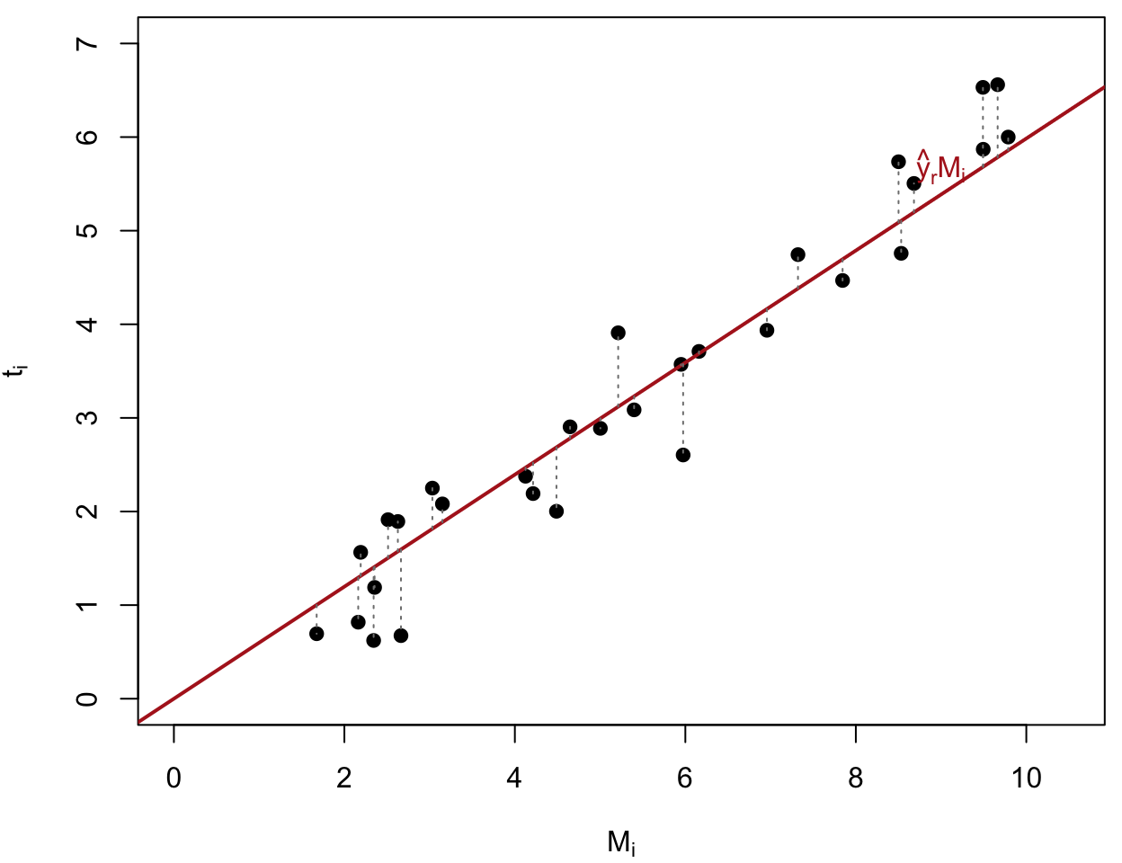
From formula (4.10) applied with x_i=M_i, y_i=t_i, and writing \hat t_{ri}=\hat{\bar y}_r M_i for the fitted value: s_r^2 = \frac{1}{n-1}\sum_{i\in\mathcal S}(t_i-\hat t_{ri})^2 \text{SE}(\hat{\bar y}_r) = \sqrt{\Big(1-\frac nN\Big)\frac{s_r^2}{n\bar M^2}} where \bar M=\sum_{i\in\mathcal S}M_i/n. The residuals t_i - \hat t_{ri} (dotted vertical segments) are typically far less variable than t_i itself.
Example: Algebra Class Test Scores
One-stage cluster samples are common in educational studies, since students are naturally clustered into classrooms or schools. From a population of 187 high-school algebra classes, an investigator takes an SRS of n=12 classes and tests every student in them for function knowledge. As with ordinary ratio estimation, \hat t_{ri}=\hat{\bar y}_r M_i is the fitted cluster total and e_i=t_i-\hat t_{ri} the residual from the line t=\hat{\bar y}_r M:
Example: Algebra Class Test Scores (Calculation)
| Class | M_i | \bar y_i | t_i | \hat t_{ri} | e_i | e_i^2 | |
|---|---|---|---|---|---|---|---|
| 23 | 20 | 61.5 | 1,230.0 | 1,251.4 | −21.4 | 456.7 | |
| 37 | 26 | 64.2 | 1,670.0 | 1,626.8 | 43.2 | 1,867.7 | |
| 38 | 24 | 58.4 | 1,402.0 | 1,501.6 | −99.6 | 9,929.2 | |
| 39 | 34 | 58.0 | 1,972.0 | 2,127.3 | −155.3 | 24,127.8 | |
| 41 | 26 | 58.0 | 1,508.0 | 1,626.8 | −118.8 | 14,109.3 | |
| 44 | 28 | 64.9 | 1,816.0 | 1,751.9 | 64.1 | 4,106.3 | |
| 46 | 19 | 55.2 | 1,048.0 | 1,188.8 | −140.8 | 19,825.4 | |
| 51 | 32 | 72.1 | 2,308.0 | 2,002.2 | 305.8 | 93,517.3 | |
| 58 | 17 | 58.2 | 989.0 | 1,063.7 | −74.7 | 5,574.9 | |
| 62 | 21 | 66.6 | 1,398.0 | 1,313.9 | 84.1 | 7,066.1 | |
| 106 | 26 | 62.3 | 1,621.0 | 1,626.8 | −5.8 | 33.4 | |
| 108 | 26 | 67.2 | 1,746.0 | 1,626.8 | 119.2 | 14,212.8 | |
| Sum | — | 299.00 | — | 18,708.00 | — | 0.00 | 194,827.04 |
The Sum row gives \sum M_i, \sum t_i, and \sum e_i^2 directly: \begin{aligned} \hat{\bar y}_r &= \frac{\sum t_i}{\sum M_i} = \frac{18{,}708}{299} = 62.57 \\[4pt] s_e^2 &= \frac{\sum e_i^2}{n-1} = \frac{194{,}827}{11} = 17{,}711.5 \\[4pt] \bar M &= \frac{299}{12} = 24.92 \\[4pt] \text{SE}(\hat{\bar y}_r) &= \sqrt{\Big(1-\frac{12}{187}\Big)\frac{s_e^2}{n\bar M^2}} = 1.49 \end{aligned}
5 A Toy Example: Why Unbiased Estimation Can Be Bad
Setup: Estimating Legs per Dog
Consider a whimsical population of just N=2 “clusters” (kennels) of dogs — kennel A with M_A=30 dogs, and kennel B with M_B=10 dogs. Every dog has exactly 4 legs, so the true population mean is trivially \bar y_U = 4 legs/dog. We take a one-stage cluster sample of n=1 kennel (each chosen with probability 1/2), observing all dogs in it.
Unbiased Estimation
Data Set 1: Kennel A Selected
t_1 = 30\times 4 = 120, \qquad \hat t_{\text{unb}} = \frac{2}{1}(120) = 240, \qquad \hat{\bar y}_{\text{unb}} = \frac{240}{30+10} = 6
Data Set 2: Kennel B Selected
t_2 = 10\times 4 = 40, \qquad \hat t_{\text{unb}} = \frac{2}{1}(40) = 80, \qquad \hat{\bar y}_{\text{unb}} = \frac{80}{30+10} = 2
\hat{\bar y}_{\text{unb}} Is Unbiased but Highly Variable
| \hat{\bar y}_{\text{unb}} | 6 | 2 |
|---|---|---|
| Probability | 1/2 | 1/2 |
E[\hat{\bar y}_{\text{unb}}] = 6\times\tfrac12 + 2\times\tfrac12 = 4 = \bar y_U \quad\text{(unbiased!)}
But \hat{\bar y}_{\text{unb}} is never actually equal to 4 — it is always off by \pm 2, because V(t_i) is huge (kennel sizes 30 vs. 10 are very different), even though every single dog has exactly 4 legs.
The Ratio Estimator Fixes This
For kennel A: \hat{\bar y}_r = \dfrac{30\times4}{30}=4. For kennel B: \hat{\bar y}_r = \dfrac{10\times4}{10}=4.
Both possible samples give exactly \hat{\bar y}_r=4=\bar y_U, so V(\hat{\bar y}_r) = 0
The ratio estimator completely cancels out the cluster-size variability that made \hat{\bar y}_{\text{unb}} so unreliable — this is why ratio estimation (not unbiased estimation) is the standard approach for unequal-size clusters.
6 Two-Stage Cluster Sampling
What Is Two-Stage Cluster Sampling?
When sampling every ssu in a selected psu is too costly, we can subsample:
- Select an SRS \mathcal S of n psus from the population of N psus.
- Select an SRS of m_i ssus from each selected psu i (this sample is \mathcal S_i).
Since we no longer observe every ssu in a sampled psu, we must estimate each psu total: \hat t_i = \sum_{j\in\mathcal S_i} \frac{M_i}{m_i}y_{ij} = M_i\bar y_i
Unbiased Estimator of the Total
\hat t_{\text{unb}} = \frac Nn \sum_{i\in\mathcal S} \hat t_i = \sum_{i\in\mathcal S}\sum_{j\in\mathcal S_i} w_{ij}y_{ij}, \qquad w_{ij} = \frac{NM_i}{nm_i}
The variance now has two sources: variability between psus, and variability from subsampling within each sampled psu: V(\hat t_{\text{unb}}) = N^2\Big(1-\frac nN\Big)\frac{S_t^2}{n} + \frac Nn \sum_{i=1}^N \Big(1-\frac{m_i}{M_i}\Big)M_i^2\frac{S_i^2}{m_i}
The first term is exactly the one-stage cluster variance; the second term is the extra cost of not observing every ssu in each sampled psu.
Ratio Estimation for Two-Stage Sampling
As before, estimating \bar y_U is a ratio estimation problem with y_i=\hat t_i=M_i\bar y_i and x_i=M_i: \hat{\bar y}_r = \frac{\sum_{i\in\mathcal S}\hat t_i}{\sum_{i\in\mathcal S}M_i} = \frac{\sum_{i\in\mathcal S}M_i\bar y_i}{\sum_{i\in\mathcal S}M_i} \hat V(\hat{\bar y}_r) = \frac{1}{\bar M^2}\Big(1-\frac nN\Big)\frac{s_r^2}{n} + \frac{1}{nN\bar M^2}\sum_{i\in\mathcal S}M_i^2\Big(1-\frac{m_i}{M_i}\Big)\frac{s_i^2}{m_i} where s_r^2 = \frac{1}{n-1}\sum_{i\in\mathcal S}(M_i\bar y_i - M_i\hat{\bar y}_r)^2. The second term is often negligible compared with the first.
Example: American Coot Egg Volumes
Data from Arnold’s (1991) study of egg size and volume of American Coot eggs in Minnedosa, Manitoba. We look at the volumes of a subsample of eggs within clutches (nests) having at least two eggs measured — the clutches are the psus, and eggs within a clutch are the ssus.
Figure: Egg Volume by Clutch
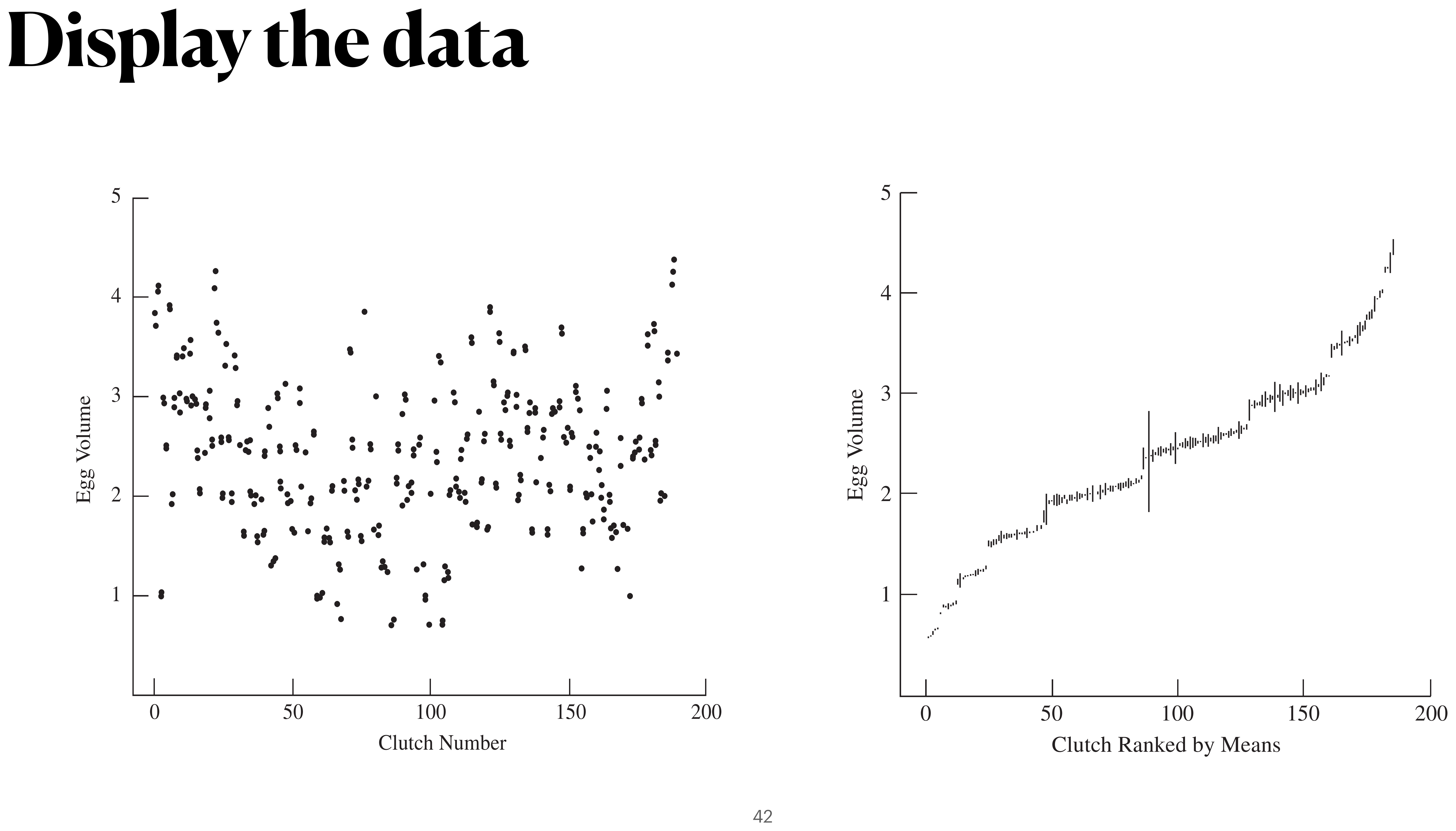
The right panel orders clutches by their mean volume, connecting the two measured eggs in each clutch — there is wide variation between clutches (clutch means climb steadily left to right), but the two eggs within a clutch usually agree closely. This indicates eggs within the same clutch are much more similar than two randomly chosen eggs from different clutches.
Example: Coots — Spreadsheet Calculation
As in the algebra example, \hat t_{ri}=\hat{\bar y}_r M_i and e_i=\hat t_i-\hat t_{ri} come from the ratio line fit to (\hat t_i, M_i) across all n=184 clutches (scroll for more rows):
| Clutch | M_i | \bar y_i | \hat t_i | \hat t_{ri} | e_i | e_i^2 | |
|---|---|---|---|---|---|---|---|
| 1 | 13 | 3.86 | 50.24 | 32.38 | 17.86 | 318.92 | |
| 2 | 13 | 4.19 | 54.52 | 32.38 | 22.15 | 490.48 | |
| 3 | 6 | 0.92 | 5.50 | 14.94 | −9.45 | 89.23 | |
| 4 | 11 | 3.00 | 32.98 | 27.40 | 5.59 | 31.20 | |
| 5 | 10 | 2.50 | 24.96 | 24.91 | 0.05 | 0.00 | |
| 6 | 13 | 3.98 | 51.80 | 32.38 | 19.42 | 377.05 | |
| 7 | 9 | 1.93 | 17.34 | 22.42 | −5.07 | 25.72 | |
| 8 | 11 | 2.96 | 32.58 | 27.40 | 5.18 | 26.84 | |
| 9 | 12 | 3.46 | 41.53 | 29.89 | 11.64 | 135.49 | |
| 10 | 11 | 2.96 | 32.58 | 27.40 | 5.18 | 26.84 | |
| 11 | 12 | 3.50 | 41.99 | 29.89 | 12.10 | 146.41 | |
| 12 | 11 | 3.00 | 33.00 | 27.40 | 5.60 | 31.38 | |
| 13 | 12 | 3.57 | 42.80 | 29.89 | 12.91 | 166.68 | |
| 14 | 11 | 2.99 | 32.85 | 27.40 | 5.45 | 29.71 | |
| 15 | 11 | 2.98 | 32.81 | 27.40 | 5.42 | 29.34 | |
| 16 | 10 | 2.41 | 24.07 | 24.91 | −0.84 | 0.70 | |
| 17 | 9 | 2.01 | 18.09 | 22.42 | −4.32 | 18.69 | |
| 18 | 10 | 2.44 | 24.37 | 24.91 | −0.53 | 0.28 | |
| 19 | 11 | 2.93 | 32.19 | 27.40 | 4.79 | 22.97 | |
| 20 | 11 | 2.95 | 32.42 | 27.40 | 5.03 | 25.29 | |
| 21 | 10 | 2.54 | 25.38 | 24.91 | 0.47 | 0.22 | |
| 22 | 13 | 4.27 | 55.50 | 32.38 | 23.12 | 534.60 | |
| 23 | 12 | 3.77 | 45.18 | 29.89 | 15.30 | 234.02 | |
| 24 | 10 | 2.56 | 25.64 | 24.91 | 0.74 | 0.54 | |
| 25 | 9 | 1.96 | 17.66 | 22.42 | −4.76 | 22.63 | |
| 26 | 12 | 3.48 | 41.79 | 29.89 | 11.90 | 141.68 | |
| 27 | 10 | 2.57 | 25.74 | 24.91 | 0.84 | 0.70 | |
| 28 | 9 | 1.96 | 17.60 | 22.42 | −4.81 | 23.16 | |
| 29 | 12 | 3.41 | 40.89 | 29.89 | 11.00 | 121.11 | |
| 30 | 11 | 2.96 | 32.51 | 27.40 | 5.11 | 26.14 | |
| 31 | 10 | 2.50 | 25.05 | 24.91 | 0.14 | 0.02 | |
| 32 | 8 | 1.56 | 12.48 | 19.92 | −7.45 | 55.43 | |
| 33 | 10 | 2.49 | 24.92 | 24.91 | 0.01 | 0.00 | |
| 34 | 10 | 2.49 | 24.87 | 24.91 | −0.04 | 0.00 | |
| 35 | 9 | 1.99 | 17.88 | 22.42 | −4.54 | 20.57 | |
| 36 | 9 | 1.93 | 17.33 | 22.42 | −5.09 | 25.91 | |
| 37 | 8 | 1.50 | 11.98 | 19.92 | −7.94 | 63.12 | |
| 38 | 9 | 1.93 | 17.41 | 22.42 | −5.01 | 25.07 | |
| 39 | 8 | 1.56 | 12.52 | 19.92 | −7.41 | 54.85 | |
| 40 | 10 | 2.41 | 24.13 | 24.91 | −0.77 | 0.60 | |
| 41 | 11 | 2.82 | 31.01 | 27.40 | 3.61 | 13.04 | |
| 42 | 7 | 1.23 | 8.64 | 17.43 | −8.80 | 77.36 | |
| 43 | 7 | 1.26 | 8.83 | 17.43 | −8.61 | 74.11 | |
| 44 | 11 | 3.03 | 33.34 | 27.40 | 5.94 | 35.28 | |
| 45 | 10 | 2.47 | 24.72 | 24.91 | −0.19 | 0.04 | |
| 46 | 9 | 2.08 | 18.68 | 22.42 | −3.73 | 13.93 | |
| 47 | 11 | 3.16 | 34.75 | 27.40 | 7.36 | 54.12 | |
| 48 | 9 | 1.93 | 17.41 | 22.42 | −5.01 | 25.07 | |
| 49 | 9 | 1.91 | 17.23 | 22.42 | −5.18 | 26.86 | |
| 50 | 8 | 1.59 | 12.74 | 19.92 | −7.19 | 51.63 | |
| 51 | 10 | 2.47 | 24.70 | 24.91 | −0.20 | 0.04 | |
| 52 | 11 | 3.04 | 33.47 | 27.40 | 6.07 | 36.90 | |
| 53 | 9 | 2.06 | 18.55 | 22.42 | −3.86 | 14.91 | |
| 54 | 10 | 2.43 | 24.26 | 24.91 | −0.65 | 0.42 | |
| 55 | 8 | 1.58 | 12.62 | 19.92 | −7.31 | 53.42 | |
| 56 | 9 | 1.90 | 17.11 | 22.42 | −5.30 | 28.12 | |
| 57 | 10 | 2.64 | 26.36 | 24.91 | 1.46 | 2.13 | |
| 58 | 6 | 0.88 | 5.27 | 14.94 | −9.68 | 93.62 | |
| 59 | 6 | 0.88 | 5.27 | 14.94 | −9.67 | 93.57 | |
| 60 | 6 | 0.90 | 5.42 | 14.94 | −9.53 | 90.78 | |
| 61 | 8 | 1.49 | 11.95 | 19.92 | −7.97 | 63.53 | |
| 62 | 8 | 1.60 | 12.78 | 19.92 | −7.15 | 51.07 | |
| 63 | 8 | 1.50 | 11.98 | 19.92 | −7.94 | 63.12 | |
| 64 | 9 | 2.04 | 18.38 | 22.42 | −4.04 | 16.29 | |
| 65 | 6 | 0.81 | 4.88 | 14.94 | −10.06 | 101.24 | |
| 66 | 7 | 1.20 | 8.43 | 17.43 | −9.00 | 81.08 | |
| 67 | 5 | 0.66 | 3.30 | 12.45 | −9.15 | 83.77 | |
| 68 | 9 | 2.06 | 18.58 | 22.42 | −3.83 | 14.70 | |
| 69 | 8 | 1.55 | 12.38 | 19.92 | −7.54 | 56.89 | |
| 70 | 12 | 3.51 | 42.16 | 29.89 | 12.28 | 150.68 | |
| 71 | 10 | 2.52 | 25.24 | 24.91 | 0.33 | 0.11 | |
| 72 | 9 | 1.98 | 17.81 | 22.42 | −4.61 | 21.25 | |
| 73 | 9 | 2.10 | 18.88 | 22.42 | −3.54 | 12.52 | |
| 74 | 8 | 1.51 | 12.08 | 19.92 | −7.85 | 61.58 | |
| 75 | 13 | 3.92 | 50.92 | 32.38 | 18.54 | 343.86 | |
| 76 | 9 | 2.09 | 18.80 | 22.42 | −3.61 | 13.04 | |
| 77 | 10 | 2.48 | 24.79 | 24.91 | −0.11 | 0.01 | |
| 78 | 8 | 1.59 | 12.69 | 19.92 | −7.24 | 52.38 | |
| 79 | 11 | 3.04 | 33.39 | 27.40 | 6.00 | 35.96 | |
| 80 | 8 | 1.58 | 12.63 | 19.92 | −7.30 | 53.23 | |
| 81 | 7 | 1.22 | 8.52 | 17.43 | −8.91 | 79.44 | |
| 82 | 7 | 1.19 | 8.32 | 17.43 | −9.11 | 83.04 | |
| 83 | 7 | 1.15 | 8.08 | 17.43 | −9.36 | 87.54 | |
| 84 | 5 | 0.58 | 2.89 | 12.45 | −9.57 | 91.50 | |
| 85 | 5 | 0.65 | 3.25 | 12.45 | −9.21 | 84.76 | |
| 86 | 9 | 2.12 | 19.05 | 22.42 | −3.36 | 11.32 | |
| 87 | 10 | 2.48 | 24.78 | 24.91 | −0.13 | 0.02 | |
| 88 | 9 | 2.35 | 21.13 | 22.42 | −1.28 | 1.64 | |
| 89 | 11 | 3.02 | 33.17 | 27.40 | 5.77 | 33.30 | |
| 90 | 9 | 1.98 | 17.86 | 22.42 | −4.56 | 20.76 | |
| 91 | 9 | 2.03 | 18.31 | 22.42 | −4.11 | 16.88 | |
| 92 | 10 | 2.41 | 24.14 | 24.91 | −0.76 | 0.59 | |
| 93 | 7 | 1.18 | 8.28 | 17.43 | −9.15 | 83.71 | |
| 94 | 10 | 2.55 | 25.46 | 24.91 | 0.55 | 0.30 | |
| 95 | 7 | 1.23 | 8.59 | 17.43 | −8.85 | 78.28 | |
| 96 | 6 | 0.88 | 5.28 | 14.94 | −9.66 | 93.34 | |
| 97 | 5 | 0.59 | 2.97 | 12.45 | −9.48 | 89.91 | |
| 98 | 9 | 1.98 | 17.81 | 22.42 | −4.61 | 21.23 | |
| 99 | 11 | 2.99 | 32.87 | 27.40 | 5.47 | 29.93 | |
| 100 | 10 | 2.37 | 23.67 | 24.91 | −1.24 | 1.53 | |
| 101 | 12 | 3.43 | 41.16 | 29.89 | 11.28 | 127.16 | |
| 102 | 5 | 0.62 | 3.08 | 12.45 | −9.37 | 87.78 | |
| 103 | 7 | 1.13 | 7.94 | 17.43 | −9.49 | 90.06 | |
| 104 | 7 | 1.12 | 7.84 | 17.43 | −9.59 | 92.04 | |
| 105 | 9 | 1.99 | 17.89 | 22.42 | −4.53 | 20.51 | |
| 106 | 11 | 3.01 | 33.13 | 27.40 | 5.73 | 32.88 | |
| 107 | 9 | 2.09 | 18.83 | 22.42 | −3.58 | 12.82 | |
| 108 | 9 | 1.96 | 17.64 | 22.42 | −4.78 | 22.83 | |
| 109 | 10 | 2.41 | 24.11 | 24.91 | −0.80 | 0.63 | |
| 110 | 9 | 1.93 | 17.39 | 22.42 | −5.03 | 25.27 | |
| 111 | 10 | 2.60 | 26.00 | 24.91 | 1.10 | 1.21 | |
| 112 | 12 | 3.63 | 43.54 | 29.89 | 13.66 | 186.46 | |
| 113 | 8 | 1.65 | 13.19 | 19.92 | −6.74 | 45.36 | |
| 114 | 8 | 1.65 | 13.18 | 19.92 | −6.74 | 45.47 | |
| 115 | 11 | 2.87 | 31.57 | 27.40 | 4.17 | 17.43 | |
| 116 | 9 | 2.12 | 19.06 | 22.42 | −3.35 | 11.23 | |
| 117 | 10 | 2.58 | 25.82 | 24.91 | 0.91 | 0.83 | |
| 118 | 8 | 1.61 | 12.85 | 19.92 | −7.08 | 50.11 | |
| 119 | 13 | 3.96 | 51.48 | 32.38 | 19.11 | 365.04 | |
| 120 | 11 | 3.16 | 34.71 | 27.40 | 7.31 | 53.43 | |
| 121 | 9 | 2.06 | 18.58 | 22.42 | −3.84 | 14.72 | |
| 122 | 12 | 3.65 | 43.83 | 29.89 | 13.94 | 194.44 | |
| 123 | 10 | 2.60 | 26.00 | 24.91 | 1.09 | 1.20 | |
| 124 | 11 | 2.93 | 32.23 | 27.40 | 4.83 | 23.36 | |
| 125 | 11 | 3.06 | 33.63 | 27.40 | 6.23 | 38.85 | |
| 126 | 10 | 2.52 | 25.21 | 24.91 | 0.31 | 0.09 | |
| 127 | 12 | 3.50 | 41.96 | 29.89 | 12.08 | 145.88 | |
| 128 | 11 | 2.99 | 32.84 | 27.40 | 5.44 | 29.60 | |
| 129 | 9 | 1.93 | 17.39 | 22.42 | −5.02 | 25.24 | |
| 130 | 9 | 2.15 | 19.38 | 22.42 | −3.03 | 9.20 | |
| 131 | 12 | 3.54 | 42.50 | 29.89 | 12.61 | 159.07 | |
| 132 | 10 | 2.65 | 26.53 | 24.91 | 1.62 | 2.63 | |
| 133 | 11 | 2.91 | 32.02 | 27.40 | 4.62 | 21.35 | |
| 134 | 8 | 1.59 | 12.69 | 19.92 | −7.23 | 52.31 | |
| 135 | 11 | 2.88 | 31.63 | 27.40 | 4.23 | 17.91 | |
| 136 | 9 | 2.10 | 18.88 | 22.42 | −3.54 | 12.50 | |
| 137 | 10 | 2.36 | 23.62 | 24.91 | −1.29 | 1.66 | |
| 138 | 10 | 2.62 | 26.24 | 24.91 | 1.33 | 1.77 | |
| 139 | 8 | 1.57 | 12.57 | 19.92 | −7.36 | 54.10 | |
| 140 | 9 | 2.05 | 18.42 | 22.42 | −3.99 | 15.95 | |
| 141 | 11 | 2.87 | 31.60 | 27.40 | 4.20 | 17.66 | |
| 142 | 11 | 2.88 | 31.73 | 27.40 | 4.33 | 18.78 | |
| 143 | 11 | 2.94 | 32.32 | 27.40 | 4.93 | 24.28 | |
| 144 | 12 | 3.73 | 44.78 | 29.89 | 14.89 | 221.85 | |
| 145 | 10 | 2.58 | 25.79 | 24.91 | 0.89 | 0.79 | |
| 146 | 10 | 2.61 | 26.10 | 24.91 | 1.20 | 1.43 | |
| 147 | 9 | 2.04 | 18.34 | 22.42 | −4.07 | 16.58 | |
| 148 | 10 | 2.61 | 26.08 | 24.91 | 1.17 | 1.38 | |
| 149 | 11 | 3.10 | 34.15 | 27.40 | 6.76 | 45.65 | |
| 150 | 11 | 2.93 | 32.19 | 27.40 | 4.79 | 22.93 | |
| 151 | 7 | 1.17 | 8.22 | 17.43 | −9.22 | 84.96 | |
| 152 | 8 | 1.57 | 12.57 | 19.92 | −7.35 | 54.03 | |
| 153 | 9 | 1.97 | 17.74 | 22.42 | −4.67 | 21.83 | |
| 154 | 10 | 2.43 | 24.26 | 24.91 | −0.64 | 0.41 | |
| 155 | 9 | 1.82 | 16.42 | 22.42 | −5.99 | 35.90 | |
| 156 | 10 | 2.56 | 25.63 | 24.91 | 0.73 | 0.53 | |
| 157 | 10 | 2.34 | 23.40 | 24.91 | −1.51 | 2.27 | |
| 158 | 9 | 2.00 | 17.99 | 22.42 | −4.42 | 19.56 | |
| 159 | 9 | 1.75 | 15.77 | 22.42 | −6.64 | 44.10 | |
| 160 | 11 | 2.99 | 32.89 | 27.40 | 5.50 | 30.22 | |
| 161 | 9 | 1.94 | 17.48 | 22.42 | −4.93 | 24.33 | |
| 162 | 8 | 1.56 | 12.46 | 19.92 | −7.46 | 55.68 | |
| 163 | 8 | 1.60 | 12.78 | 19.92 | −7.15 | 51.09 | |
| 164 | 7 | 1.18 | 8.27 | 17.43 | −9.16 | 83.98 | |
| 165 | 10 | 2.44 | 24.37 | 24.91 | −0.54 | 0.29 | |
| 166 | 8 | 1.65 | 13.22 | 19.92 | −6.71 | 45.01 | |
| 167 | 8 | 1.61 | 12.84 | 19.92 | −7.08 | 50.19 | |
| 168 | 6 | 0.88 | 5.29 | 14.94 | −9.65 | 93.09 | |
| 169 | 10 | 2.39 | 23.85 | 24.91 | −1.05 | 1.11 | |
| 170 | 10 | 2.48 | 24.83 | 24.91 | −0.08 | 0.01 | |
| 171 | 10 | 2.51 | 25.15 | 24.91 | 0.24 | 0.06 | |
| 172 | 11 | 2.98 | 32.80 | 27.40 | 5.40 | 29.16 | |
| 173 | 10 | 2.35 | 23.46 | 24.91 | −1.44 | 2.09 | |
| 174 | 12 | 3.62 | 43.43 | 29.89 | 13.55 | 183.48 | |
| 175 | 10 | 2.43 | 24.34 | 24.91 | −0.57 | 0.32 | |
| 176 | 12 | 3.75 | 45.03 | 29.89 | 15.14 | 229.35 | |
| 177 | 10 | 2.53 | 25.27 | 24.91 | 0.37 | 0.14 | |
| 178 | 11 | 3.10 | 34.11 | 27.40 | 6.72 | 45.10 | |
| 179 | 9 | 1.94 | 17.46 | 22.42 | −4.95 | 24.52 | |
| 180 | 9 | 1.95 | 17.52 | 22.42 | −4.90 | 23.97 | |
| 181 | 12 | 3.45 | 41.44 | 29.89 | 11.55 | 133.46 | |
| 182 | 13 | 4.22 | 54.86 | 32.38 | 22.48 | 505.40 | |
| 183 | 13 | 4.41 | 57.39 | 32.38 | 25.02 | 625.75 | |
| 184 | 12 | 3.48 | 41.81 | 29.89 | 11.92 | 142.20 | |
| Sum | — | 1,757.00 | — | 4,375.95 | — | 0.00 | 11,439.58 |
Example: Coots — Results
The Sum row gives \sum M_i, \sum \hat t_i, and \sum e_i^2: \hat{\bar y}_r = \frac{\sum \hat t_i}{\sum M_i} = \frac{4375.95}{1757} = 2.49, \qquad s_r^2 = \frac{\sum e_i^2}{n-1} = \frac{11{,}439.58}{183} = 62.51, \qquad \bar M = \frac{1757}{184}=9.549
Since the total number of clutches N is unknown but presumably very large, the psu-level fpc (1-n/N)\approx 1, and the second (within-clutch) variance term is negligible relative to the first: \text{SE}(\hat{\bar y}_r) = \frac{1}{9.549}\sqrt{\frac{62.51}{184}} = 0.061, \qquad \widehat{\text{CV}}(\hat{\bar y}_r) = \frac{0.061}{2.49} = 0.0245