STAT 348 Sampling Techniques
Introduction to Unequal Probability Sampling
1 Introduction to Unequal Probability Sampling
Textbook sections:
- 6.1–6.3 in Lohr’s book (not covering UPS without replacement)
- 8.9 and 9.7 in Scheaffer et al., titled “Cluster Sampling with Probabilities Proportional to Size”
Introductory Example
O’Brien et al. (1995) sampled nursing home residents in the Philadelphia area to determine residents’ preferences on life-sustaining treatments (CPR, hospital transfer, feeding tubes). The target population was all residents of 294 licensed nursing homes, with 37,652 beds total — before sampling, only the number of beds was known, not the number of residents.
In a cluster sample with equal probabilities, a nursing home with 20 beds is just as likely to be chosen as one with 1000 beds — wasting the fact that we already know home size, and that resident counts (and hence answers) are tied to home size.
A Toy Example
A town has four supermarkets, ranging in size from 100\,\text{m}^2 to 1000\,\text{m}^2. We want to estimate total sales across the four stores last month, but can only afford to sample one store. Let \psi_i = P(\text{Store } i \text{ selected}).
Scheme 1: Probabilities Proportional to Size (PPS)
Since Store D accounts for 10/16 of the total floor area, we sample it with probability 10/16:
| Store | Size (M_i) | \psi_i | t_i (thousands) |
|---|---|---|---|
| A | 100 | 1/16 | 11 |
| B | 200 | 2/16 | 20 |
| C | 300 | 3/16 | 24 |
| D | 1000 | 10/16 | 245 |
| Total | 1600 | 1 | 300 |
We could realize this design with 16 numbered cards: card 1 \to A; cards 2–3 \to B; cards 4–6 \to C; cards 7–16 \to D.
Estimation for Scheme 1
Since only one store is sampled, define the Hansen-Hurwitz estimator \hat t_\psi = t_i/\psi_i for the selected store i. The Sum row gives E[\hat t_\psi] and V[\hat t_\psi] directly:
| Sample | \psi_i | t_i | \hat t_\psi | \psi_i\hat t_\psi | (\hat t_\psi-t)^2 | \psi_i(\hat t_\psi-t)^2 |
|---|---|---|---|---|---|---|
| \{A\} | 1/16 | 11 | 176 | 11 | 15,376 | 961 |
| \{B\} | 2/16 | 20 | 160 | 20 | 19,600 | 2,450 |
| \{C\} | 3/16 | 24 | 128 | 24 | 29,584 | 5,547 |
| \{D\} | 10/16 | 245 | 392 | 245 | 8,464 | 5,290 |
| Sum | 1 | 300 | 300 | 14,248 |
\begin{aligned} E[\hat t_\psi] &= \sum_{i=1}^N \psi_i\hat t_\psi = 300 = t \\[4pt] V[\hat t_\psi] &= \sum_{i=1}^N \psi_i(\hat t_\psi-t)^2 = 14{,}248 \end{aligned}
\hat t_\psi is always unbiased, because in general E[\hat t_\psi]=\sum_{i=1}^N \psi_i\dfrac{t_i}{\psi_i}=t.
Scheme 2: SRS with Simple (Unbiased) Estimation
Now suppose instead we take an SRS of size 1, so \psi_i=1/4 for every store (and 1/\psi_i=4=N). The Sum row gives V[\hat t_{\text{SRS}}] directly:
| Sample | \psi_i | t_i | \hat t_\psi | (\hat t_\psi-t)^2 | \psi_i(\hat t_\psi-t)^2 |
|---|---|---|---|---|---|
| \{A\} | 1/4 | 11 | 44 | 65,536 | 16,384 |
| \{B\} | 1/4 | 20 | 80 | 48,400 | 12,100 |
| \{C\} | 1/4 | 24 | 96 | 41,616 | 10,404 |
| \{D\} | 1/4 | 245 | 980 | 462,400 | 115,600 |
| Sum | 1 | 154,488 |
\begin{aligned} E[\hat t_{\text{SRS}}] &= 300 = t \\[4pt] V[\hat t_{\text{SRS}}] &= \sum_{i} \psi_i(\hat t_\psi-t)^2 = 154{,}488 \end{aligned}
\hat t_{\text{SRS}} is still unbiased, but this is over ten times larger than the PPS design’s variance of 14,248!
The PPS design uses auxiliary information: store size is known and related to sales, and the design exploits this. If Store D were selected under SRS, its huge sales total gets multiplied by N=4 (since it represents only itself), producing a wildly unstable estimate.
Scheme 2: SRS with Ratio Estimation
Alternatively, keep the SRS of size 1 but use ratio estimation with x_i=M_i (known total M_0=1600), \hat t_r = \dfrac{t_i}{M_i}\cdot M_0. The Sum row gives \sum(\hat t_r-t)^2 directly:
| Store | M_i | t_i | \hat t_r | \hat t_r-t | (\hat t_r-t)^2 |
|---|---|---|---|---|---|
| A | 100 | 11 | 176 | -124 | 15,376 |
| B | 200 | 20 | 160 | -140 | 19,600 |
| C | 300 | 24 | 128 | -172 | 29,584 |
| D | 1000 | 245 | 392 | 92 | 8,464 |
| Sum | 1600 | 300 | 856 | 73,024 |
\begin{aligned} E(\hat t_r) &= \frac{856}{4} = 214 \quad(\ne 300,\ \text{biased!}) \\[4pt] \text{MSE}(\hat t_r) &= \frac{\sum(\hat t_r-t)^2}{4} = \frac{73{,}024}{4} = 18{,}256 \end{aligned}
Ratio Estimation vs. Unequal Probability Sampling
Notice the four \hat t_r values (176, 160, 128, 392) are numerically identical to the PPS estimates \hat t_\psi from Scheme 1! But averaged with the equal SRS probabilities (1/4 each) rather than the size-based PPS probabilities, they give a biased result (214, not 300).
- Ratio estimation is an estimating method that exploits the correlation between t_i and M_i after an SRS is drawn.
- Unequal probability sampling is a sampling design that exploits the same correlation before the sample is drawn, by choosing \psi_i\propto M_i.
2 Unequal Probability Sampling with Replacement (UPSWR)
How to Do Unequal Probability Sampling?
Suppose n>1 and we sample with replacement: sampling with replacement means the selection probabilities do not change after the first draw. Let \psi_i = P(\text{select unit } i \text{ on any given draw}).
The idea: draw n psus with replacement (some psus may be drawn more than once). For each draw, estimate the population total using the single-draw estimator from before; average the n (independent) estimates.
A common choice, probabilities proportional to size (PPS): \psi_i = \frac{M_i}{\sum_{k=1}^N M_k}
Drawing Probabilities in Practice
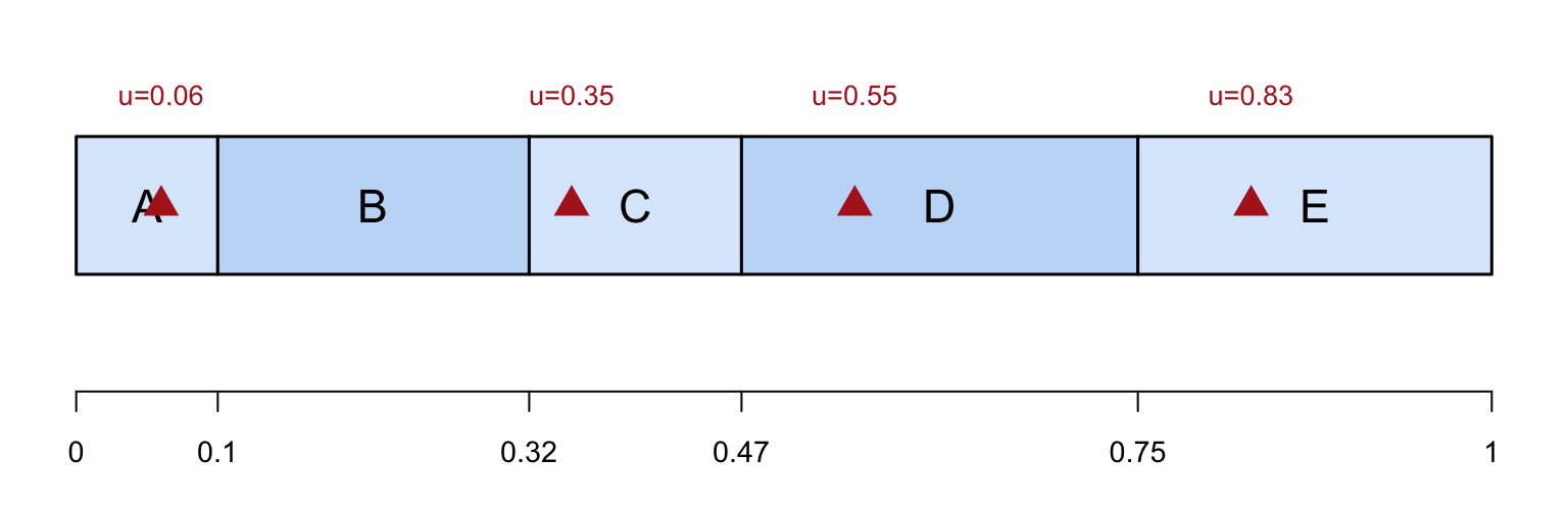
Figure 1
Divide [0,1] into segments of length \psi_1,\ldots,\psi_N. Draw a random number u\sim\text{Uniform}(0,1) (red triangles); whichever segment u falls into determines the selected unit. In R: sample(1:N, size = n, prob = psi, replace = TRUE).
Notation for the Sample \mathcal R
Because we sample with replacement, the sample may contain the same psu more than once. Let \mathcal R (not \mathcal S) denote the multiset of n draws, including repeats. For example, with the supermarket population, a sample of size n=10 might be \mathcal R = \{D,D,D,C,C,D,C,A,B,B\}.
The Hansen-Hurwitz Estimator
Let u_i = t_i/\psi_i. We saw that for a single draw, u_i is an unbiased estimator of t. Sampling n psus with replacement gives n independent copies, which we average: \hat t_\psi = \frac1n \sum_{i\in\mathcal R} \frac{t_i}{\psi_i} = \frac1n\sum_{i\in\mathcal R} u_i = \bar u
The estimated variance: \hat V(\hat t_\psi) = \frac1n\cdot\frac{1}{n-1}\sum_{i\in\mathcal R}\Big(\frac{t_i}{\psi_i}-\hat t_\psi\Big)^2
Why \hat t_\psi Is Unbiased: the IID View
Let u_j^* denote the value of u_i=t_i/\psi_i for the jth draw (not the jth population unit) — so \hat t_\psi = \frac1n\sum_{j=1}^n u_j^*=\bar u^*. Since draws are independent and identically distributed, E(u_j^*) = \sum_{i=1}^N u_i\psi_i = \sum_{i=1}^N \frac{t_i}{\psi_i}\psi_i = \sum_{i=1}^N t_i = t V(u_j^*) = \sum_{i=1}^N \psi_i(u_i-t)^2 = \sum_{i=1}^N \psi_i\Big(\frac{t_i}{\psi_i}-t\Big)^2
Since \hat t_\psi is the mean of n IID copies of u_j^*: E(\hat t_\psi) = E(u_j^*) = t, \qquad V(\hat t_\psi) = \frac{V(u_j^*)}{n} = \frac1n\sum_{i=1}^N \psi_i\Big(\frac{t_i}{\psi_i}-t\Big)^2
Note
There is no finite population correction — the n draws are independent (with replacement), unlike SRS without replacement.
Ratio Estimation for the ssu-Level Mean
We estimate the population mean \bar y_U = t/M_0 by \hat{\bar y}_\psi = \frac{\hat t_\psi}{\hat M_{0\psi}}, \qquad \hat M_{0\psi} = \frac1n\sum_{i\in\mathcal R}\frac{M_i}{\psi_i}
Using Chapter 4’s ratio-estimation results with y_i=t_i/\psi_i and x_i=M_i/\psi_i: \hat V(\hat{\bar y}_\psi) = \frac{1}{(\hat M_{0\psi})^2}\cdot\frac1n\cdot\frac{1}{n-1}\sum_{i\in\mathcal R}\Big(\frac{t_i}{\psi_i}-\hat{\bar y}_\psi\frac{M_i}{\psi_i}\Big)^2
Again, no fpc is needed, since sampled psus are drawn independently.
3 Example: College Statistics Classes
Setup
A college has 15 introductory statistics classes, with a total of 647 students. We sample n=5 classes with replacement, with probability proportional to M_i (class size), so \psi_i = M_i/647. We then survey every student in each sampled class about hours spent studying last week.
| Class | M_i | \psi_i |
|---|---|---|
| 1 | 44 | 0.0680 |
| 5 | 76 | 0.1175 |
| 12 | 24 | 0.0371 |
| 14 | 100 | 0.1546 |
| \vdots | \vdots | \vdots |
| Total | 647 | 1 |
Classes are drawn using cumulative ranges of M_i (Lahiri’s method): class 1 gets numbers 1–44, class 2 gets 45–77, and so on up to class 15.
Sample and Estimate of the Total
Suppose the sample (with repeats) is \mathcal R = \{12, 14, 14, 5, 1\}, with class totals t_i (total hours studying, summed over all students). Writing u_i=t_i/\psi_i, the Sum row gives \sum u_i and \sum(u_i-\hat t_\psi)^2 directly:
| Class | \psi_i | t_i | u_i=t_i/\psi_i | u_i-\hat t_\psi | (u_i-\hat t_\psi)^2 |
|---|---|---|---|---|---|
| 12 | 24/647 | 75 | 2021.875 | 272.861 | 74,452.9 |
| 14 | 100/647 | 203 | 1313.410 | -435.604 | 189,751.2 |
| 14 | 100/647 | 203 | 1313.410 | -435.604 | 189,751.2 |
| 5 | 76/647 | 191 | 1626.013 | -123.001 | 15,129.3 |
| 1 | 44/647 | 168 | 2470.364 | 721.349 | 520,344.8 |
| Sum | 8745.07 | 989,429.3 |
\begin{aligned} \hat t_\psi &= \frac{\sum u_i}{n} = \frac{8745.07}{5} = 1749.014 \\[4pt] s^2 &= \frac{\sum(u_i-\hat t_\psi)^2}{n-1} = \frac{989{,}429.3}{4} = 247{,}357.3 \\[4pt] \text{SE}(\hat t_\psi) &= \sqrt{\frac{s^2}{n}} = \sqrt{\frac{247{,}357.3}{5}} = 222.42 \end{aligned}
Estimate of Hours per Student
Since \psi_i = M_i/647 exactly, M_i/\psi_i = 647 for every sampled class, so \hat M_{0\psi} = M_0 = 647 exactly. The average hours studied per student: \begin{aligned} \hat{\bar y}_\psi &= \frac{1749.014}{647} = 2.70 \text{ hours} \\[4pt] \text{SE}(\hat{\bar y}_\psi) &= \frac{222.42}{647} = 0.34 \text{ hours} \end{aligned}
4 One-Stage Cluster Sampling with PPS
A Useful Simplification
When \psi_i = M_i/M_0 (PPS), then u_i = t_i/\psi_i = t_i\cdot(M_0/M_i)=\bar y_i\cdot M_0, where \bar y_i=t_i/M_i is the ith cluster’s own mean. So: \hat{\bar y}_{\text{pps}} = \frac{\hat t_\psi}{M_0} = \frac1n\sum_{i\in\mathcal R} \bar y_i \text{SE}(\hat{\bar y}_{\text{pps}}) = \frac{\text{SE}(\hat t_\psi)}{M_0} = \sqrt{\frac1n\cdot\frac{\sum_{i\in\mathcal R}(\bar y_i-\hat{\bar y}_{\text{pps}})^2}{n-1}}
Under PPS, we don’t need to weight the cluster means by M_i/\sum M_i at all — they can simply be averaged!
Example: College Classes, Revisited with the PPS Shortcut
| Class | \bar y_i = t_i/M_i |
|---|---|
| 12 | 75/24 = 3.13 |
| 14 | 203/100 = 2.03 |
| 14 | 203/100 = 2.03 |
| 5 | 191/76 = 2.51 |
| 1 | 168/44 = 3.81 |
| Sum | 13.51 |
\begin{aligned} \hat{\bar y}_{\text{pps}} &= \frac{\sum \bar y_i}{5} = \frac{13.51}{5} = 2.70 \\[4pt] \text{SE}(\hat{\bar y}_{\text{pps}}) &= 0.34 \end{aligned}
Identical to the weighted calculation on the previous slide — but computed directly as the mean and SE of the five class averages.
5 Review: SRS-of-Clusters vs. PPS
Ratio Estimation for Cluster Sampling with SRS
Recall from cluster sampling: if psus are instead drawn by an ordinary SRS (not PPS with replacement), the ratio estimator is \hat{\bar y}_r = \frac{\sum_{i\in\mathcal S} \hat t_i}{\sum_{i\in\mathcal S} M_i} = \frac{\sum_{i\in\mathcal S} M_i\bar y_i}{\sum_{i\in\mathcal S} M_i} with estimated variance (including a finite-population correction) \hat V(\hat{\bar y}_r) = \frac{1}{\bar M^2}\Big(1-\frac nN\Big)\frac{s_r^2}{n} + \frac{1}{nN\bar M^2}\sum_{i\in\mathcal S}M_i^2\Big(1-\frac{m_i}{M_i}\Big)\frac{s_i^2}{m_i}
Key Contrast
| SRS of psus + ratio estimation | PPS with replacement | |
|---|---|---|
| Selection | equal probability | \psi_i \propto M_i |
| Point estimator | \hat{\bar y}_r (ratio, slightly biased) | \hat{\bar y}_\psi (Hansen-Hurwitz ratio, still approx.) |
| Finite population correction | yes, (1-n/N) | no — draws are independent |
| Weighting of cluster means | by M_i/\sum M_i | no weighting needed if \psi_i\propto M_i |
Both approaches exploit the same correlation between t_i and M_i, but PPS builds it into the design, giving the cleanest formulas when \psi_i\propto M_i exactly.
6 Two-Stage Cluster Sampling with Replacement
Setup
Now suppose that, instead of observing every ssu in a selected psu, we take a subsample. Let Q_i be the number of times psu i occurs in \mathcal R; if Q_i>0, we draw a different, independent subsample each time psu i is selected (unlike one-stage sampling, where a repeated psu just contributes the same observed total again). For the jth subsample from psu i (j=1,\ldots,Q_i), let \hat t_{ij} estimate t_i, with E[\hat t_{ij}]=t_i.
Estimators for the Total
\hat t_\psi = \frac1n \sum_{i=1}^N\sum_{j=1}^{Q_i} \frac{\hat t_{ij}}{\psi_i} \hat V(\hat t_\psi) = \frac1n\cdot\frac{1}{n-1}\sum_{i=1}^N\sum_{j=1}^{Q_i}\Big(\frac{\hat t_{ij}}{\psi_i}-\hat t_\psi\Big)^2
(If Q_i=0 for some psu, that psu simply contributes no terms.) Because sampling is with replacement, it’s possible to draw more than one independent subsample from the same psu — so this variance estimator automatically captures both the between-psu variability and the within-psu subsampling variability.
Estimator for the ssu-Level Mean
\hat{\bar y}_\psi = \frac{\hat t_\psi}{\hat M_{0\psi}}, \qquad \hat M_{0\psi} = \frac1n\sum_{i\in\mathcal R}\frac{M_i}{\psi_i} \hat V(\hat{\bar y}_\psi) = \frac{1}{(\hat M_{0\psi})^2}\cdot\frac1n\cdot\frac{1}{n-1}\sum_{i=1}^N\sum_{j=1}^{Q_i}\Big(\frac{\hat t_{ij}}{\psi_i}-\hat{\bar y}_\psi\frac{M_i}{\psi_i}\Big)^2
If an SRS of m_i ssus is taken within psu i, the overall sampling weight for ssu j in psu i becomes w_{ij} = \frac{1}{n\psi_i}\cdot\frac{M_i}{m_i}
Example: Hours Spent Studying, Subsampled
Instead of surveying every student, we now subsample 5 students per class (class 14 is selected twice, with a different subsample of 5 each time). Writing u_i=\hat t_i/\psi_i, the Sum row gives \sum u_i and \sum(u_i-\hat t_\psi)^2 directly:
| Class | M_i | \psi_i | \bar y_i | \hat t_i | u_i | e_i=u_i-\hat t_\psi | e^2_i |
|---|---|---|---|---|---|---|---|
| 12 | 24 | 0.0371 | 2.4 | 57.6 | 1552.8 | -64.7 | 4,186.1 |
| 14 | 100 | 0.1546 | 1.6 | 160.0 | 1035.2 | -582.3 | 339,073.3 |
| 14 | 100 | 0.1546 | 2.0 | 200.0 | 1294.0 | -323.5 | 104,652.2 |
| 5 | 76 | 0.1175 | 2.8 | 212.8 | 1811.6 | 194.1 | 37,674.8 |
| 1 | 44 | 0.0680 | 3.7 | 162.8 | 2393.9 | 776.4 | 602,797.0 |
| Sum | 8087.5 | 0 | 1,088,383 |
\begin{aligned} \hat t_\psi &= \frac{8087.5}{5} = 1617.5 \\[4pt] s^2 &= \frac{1{,}088{,}383}{4} = 272{,}095.8 \\[4pt] \text{SE}(\hat t_\psi) &= \sqrt{\frac{s^2}{5}} = 233.28\\[4pt] \hat{\bar y}_\psi &= \frac{1617.5}{647} = 2.5\text{ h} \\[4pt] \text{SE}(\hat{\bar y}_\psi) &= \frac{233.28}{647} = 0.36\text{ h} \end{aligned}
Compared with the full-census example (\hat{\bar y}_\psi=2.70, \text{SE}=0.34), subsampling gives a similar point estimate at a somewhat higher SE — the price of observing fewer students per class.
7 Weights in Unequal-Probability Sampling
General Weight Formula
For sampling without replacement, the weight is the reciprocal of the inclusion probability, 1/E[Z_i]. For sampling with replacement, we use the first-stage weight w_i = \frac{1}{\text{expected number of hits}} = \frac{1}{E[Q_i]} = \frac{1}{n\psi_i}
For one-stage cluster sampling (every ssu observed each time psu i is hit), w_{ij}=w_i=1/(n\psi_i) for every ssu j in psu i, and \hat t_\psi = \sum_{i\in\mathcal R}\sum_{j=1}^{M_i} w_{ij}y_{ij}, \qquad \hat{\bar y}_\psi = \frac{\sum_{i\in\mathcal R}\sum_{j=1}^{M_i} w_{ij}y_{ij}}{\sum_{i\in\mathcal R}\sum_{j=1}^{M_i} w_{ij}}
For two-stage sampling with an SRS of m_i ssus per selected psu, the weight picks up an extra factor M_i/m_i for the subsampling stage, exactly as in ordinary two-stage cluster sampling.