Brief Introduction of Neural Networks
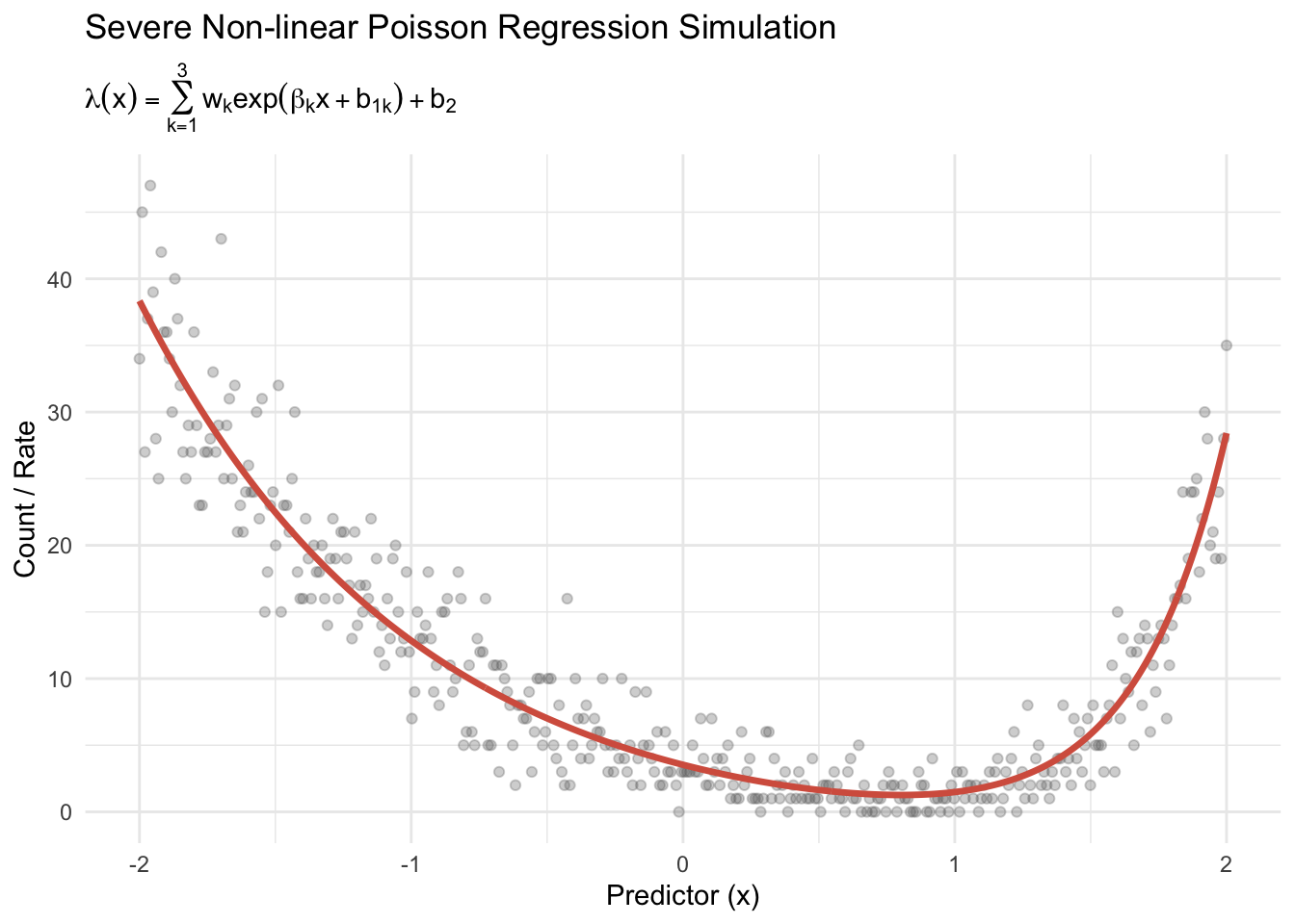
1 Non-linear Poisson Regression
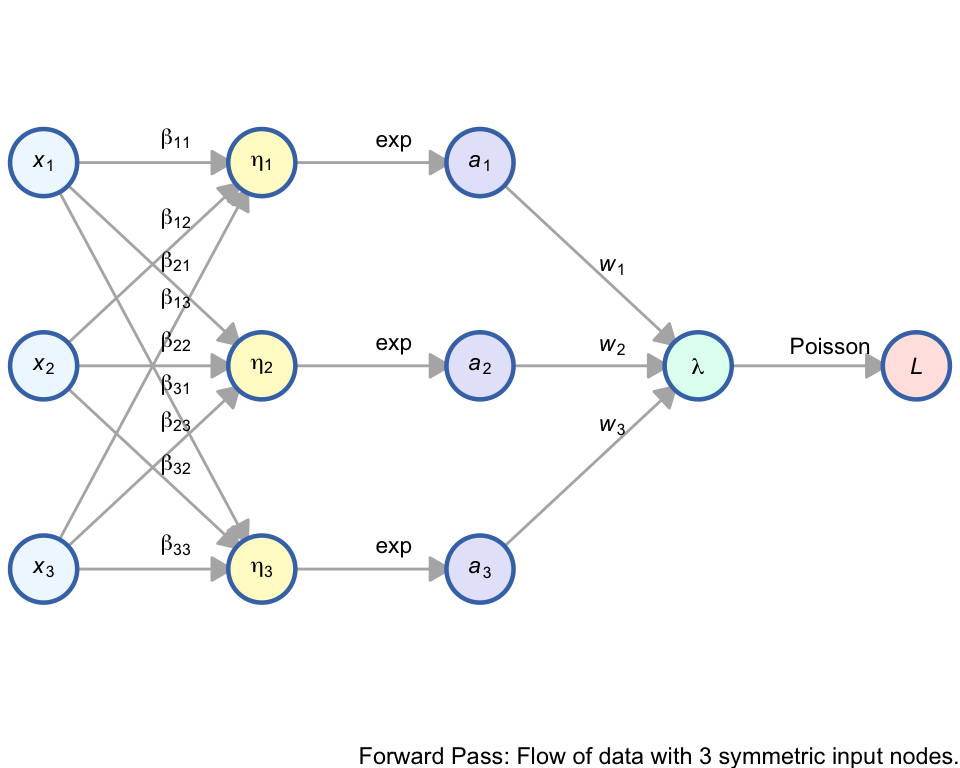
In this architecture, we extend the standard Poisson GLM by introducing a hidden layer with \(m\) units. This allows the model to learn non-linear combinations of the inputs before predicting the rate parameter \(\lambda\).
1.1 Mathematical Description
The model assumes the response variable \(y\) follows a Poisson distribution: \(y \sim \text{Poisson}(\lambda)\).
1.1.1 The Forward Pass
- Hidden Layer (Linear): \(\eta_k = \sum_{i=1}^{p} \beta_{ki} x_i + b_{1,k}\)
- Activation: \(a_k = \exp(\eta_k)\)
- Output Layer: \(\lambda = \sum_{k=1}^{m} w_k a_k + b_2\)
- Poisson Loss: \(L = \lambda - y \ln(\lambda)\)
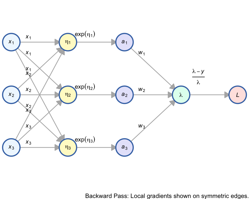
1.2 Computational Gradient Graph
In the gradient network, we compute the partial derivatives. The gradient for the hidden weight \(\beta_{ki}\) is: \[\frac{\partial L}{\partial \beta_{ki}} = x_i \cdot \exp(\eta_k) \cdot w_k \cdot \frac{\lambda - y}{\lambda}\]
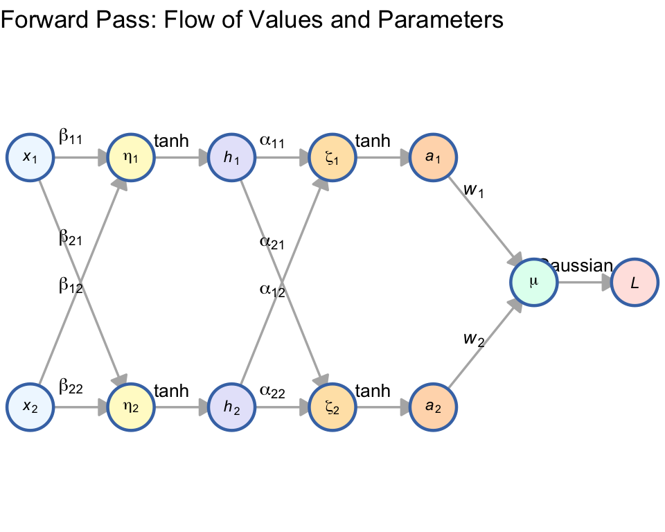
2 Neural Network: Forward and Backward Computational Graphs
2.1 The Forward Pass: Computing \(L\) from \(x\)
In the forward pass, information flows from the inputs to the loss. The edges represent the parameters (weights) and functions that transform the data.
2.1.1 Mathematical Description
For a single observation:
Layer 1: \(\eta = \mathbf{B}x + b_1 \rightarrow h = \tanh(\eta)\)
Layer 2: \(\zeta = \mathbf{A}h + b_2 \rightarrow a = \tanh(\zeta)\)
Output: \(\mu = w^T a + b_3\)
Loss: \(L = \frac{(y - \mu)^2}{2\sigma^2}\) (Gaussian Negative Log-Likelihood)
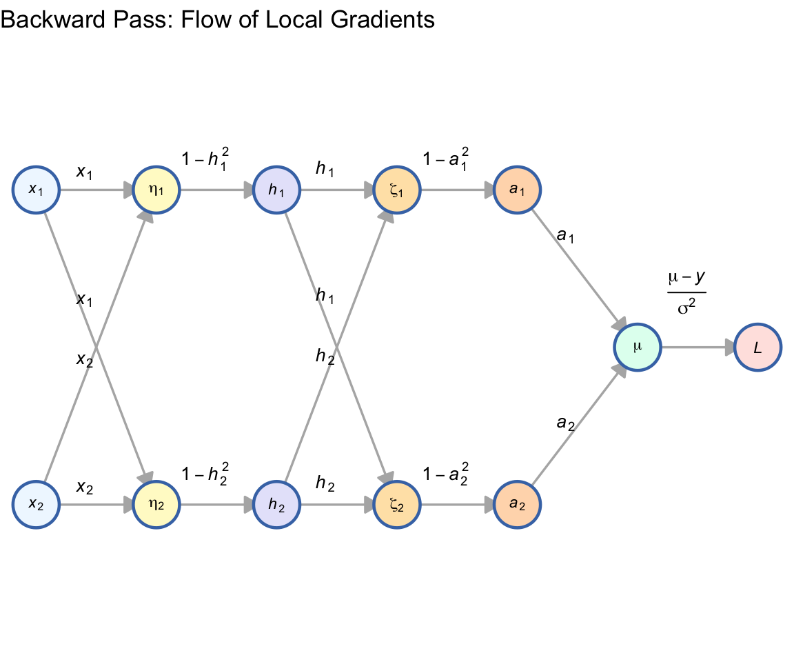
2.2 The Backward Pass: Gradient Network
In the gradient network, edges represent the local derivatives. The gradient of any node is the sum of the products of all paths leading to the loss.
2.2.1 The “Sum of Paths” Rule
To find \(\frac{\partial L}{\partial h_j}\), we sum the branches going into the next layer: \[\frac{\partial L}{\partial h_j} = \sum_{k} \left( \frac{\partial \zeta_k}{\partial h_j} \cdot \frac{\partial L}{\partial \zeta_k} \right)\]