Generate Simulated Data with Factor Analysis Model

This function generates inputs X given by the response variable y using a multivariate normal model.

gendata_FAM(n, muj, A, sd_g = 0, stdx = FALSE)

Arguments

n	Number of observations.
muj	C by p matrix, with row c representing y = c, and column j representing \(x_j\). Used to specify y.
A	Factor loading matrix of size p by p, see details.
sd_g	Numeric value indicating noise level \(\delta\), see details.
stdx	Logical; if TRUE, data X is standardized to have mean = 0 and sd = 1.

Value

A list contains input matrix X, response variables y, covariate matrix SGM and muj (standardized if stdx = TRUE).

Details

The means of each covariate \(x_j\) depend on y specified by the matrix muj; the covariate matrix \(\Sigma\) of the multivariate normal is equal to \(AA^t\delta^2I\), where A is the factor loading matrix and \(\delta\) is the noise level.

See also

gendata_MLR

Examples

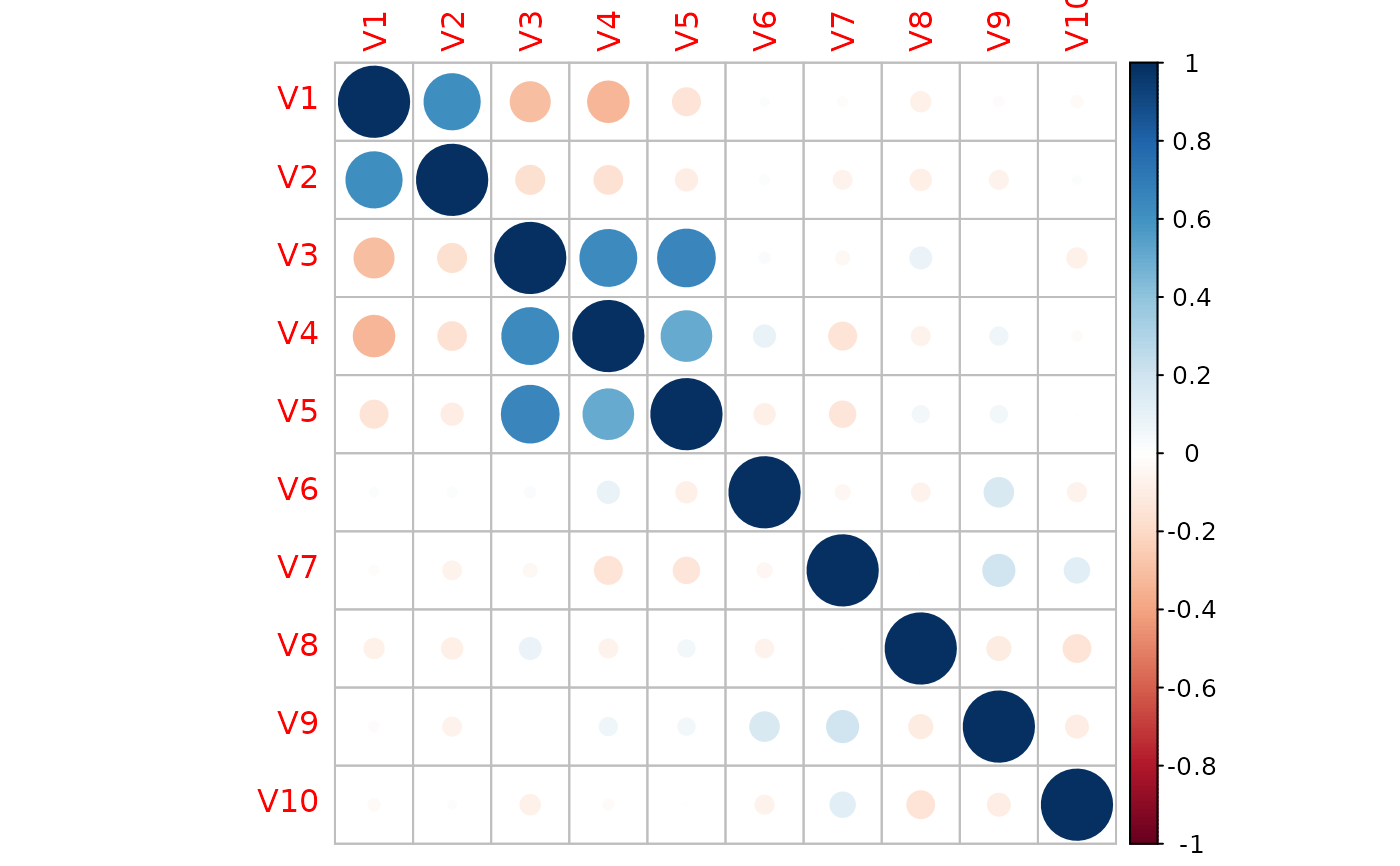
## feature #1: marginally related feature
## feature #2: marginally unrelated feature, but feature #2 is correlated with feature #1
## feature #3-5: marginally related features and also internally correlated
## feature #6-10: noise features without relationship with the y

set.seed(12345)
n <- 100
p <- 10

means <- rbind(
  c(0, 1, 0),
  c(0, 0, 0),
  c(0, 0, 1),
  c(0, 0, 1),
  c(0, 0, 1)
) * 2

means <- rbind(means, matrix(0, p - 5, 3))

A <- diag(1, p)
A[1:5, 1:3] <- rbind(
  c(1, 0, 0),
  c(2, 1, 0),
  c(0, 0, 1),
  c(0, 0, 1),
  c(0, 0, 1)
)

dat <- gendata_FAM(n, means, A, sd_g = 0.5, stdx = TRUE)
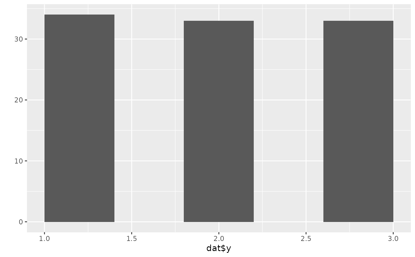
ggplot2::qplot(dat$y, bins = 6)
corrplot::corrplot(cor(dat$X))