Multinomial Logistic Regression with Heavy-Tailed Priors
Longhai Li and Steven Liu
2025-12-14
Source:vignettes/simu.Rmd
simu.RmdData Generation
Load the necessary libraries:
library(HTLR)
library(bayesplot)
#> This is bayesplot version 1.15.0
#> - Online documentation and vignettes at mc-stan.org/bayesplot
#> - bayesplot theme set to bayesplot::theme_default()
#>    * Does _not_ affect other ggplot2 plots
#>    * See ?bayesplot_theme_set for details on theme setting
The description of the dataset generating scheme is found from Li and Yao (2018).
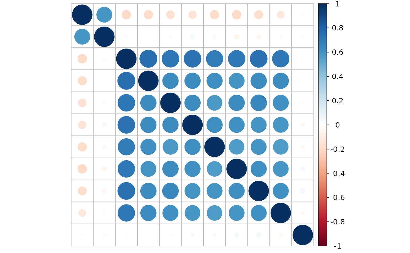
There are 4 groups of features:
feature #1: marginally related feature
feature #2: marginally unrelated feature, but feature #2 is correlated with feature #1
feature #3 - #10: marginally related features and also internally correlated
feature #11 - #2000: noise features without relationship with the y
SEED <- 123

n <- 510
p <- 2000

means <- rbind(
  c(0, 1, 0),
  c(0, 0, 0),
  c(0, 0, 1),
  c(0, 0, 1),
  c(0, 0, 1),
  c(0, 0, 1),
  c(0, 0, 1),
  c(0, 0, 1),
  c(0, 0, 1),
  c(0, 0, 1)
) * 2

means <- rbind(means, matrix(0, p - 10, 3))

A <- diag(1, p)

A[1:10, 1:3] <-
  rbind(
    c(1, 0, 0),
    c(2, 1, 0),
    c(0, 0, 1),
    c(0, 0, 1),
    c(0, 0, 1),
    c(0, 0, 1),
    c(0, 0, 1),
    c(0, 0, 1),
    c(0, 0, 1),
    c(0, 0, 1)
  )

set.seed(SEED)
dat <- gendata_FAM(n, means, A, sd_g = 0.5, stdx = TRUE)
str(dat)
#> List of 4
#>  $ X  : num [1:510, 1:2000] -0.684 0.912 -0.997 -1.262 0.613 ...
#>   ..- attr(*, "dimnames")=List of 2
#>   .. ..$ : NULL
#>   .. ..$ : chr [1:2000] "V1" "V2" "V3" "V4" ...
#>  $ muj: num [1:2000, 1:3] -0.456 0 -0.456 -0.376 -0.376 ...
#>  $ SGM: num [1:2000, 1:2000] 0.584 0.597 0 0 0 ...
#>  $ y  : int [1:510] 1 2 3 1 2 3 1 2 3 1 ...
Look at the correlation between features:
Split the data into training and testing sets:
set.seed(SEED)
dat <- split_data(dat$X, dat$y, n.train = 500)
str(dat)
#> List of 4
#>  $ x.tr: num [1:500, 1:2000] -0.903 -0.632 1.111 1.446 -0.43 ...
#>   ..- attr(*, "dimnames")=List of 2
#>   .. ..$ : NULL
#>   .. ..$ : chr [1:2000] "V1" "V2" "V3" "V4" ...
#>  $ y.tr: int [1:500] 1 1 2 2 3 3 3 1 2 1 ...
#>  $ x.te: num [1:10, 1:2000] 1.955 1.188 -0.942 -1.387 0.879 ...
#>   ..- attr(*, "dimnames")=List of 2
#>   .. ..$ : NULL
#>   .. ..$ : chr [1:2000] "V1" "V2" "V3" "V4" ...
#>  $ y.te: int [1:10] 2 2 3 3 2 3 1 2 2 2
Model Fitting
Fit a HTLR model with all default settings:
set.seed(SEED)
system.time(
  fit.t <- htlr(dat$x.tr, dat$y.tr)
)
#>    user  system elapsed
#> 240.234   0.164  60.703
print(fit.t)
#> Fitted HTLR model
#>
#>  Data:
#>
#>   response:  3-class
#>   observations:  500
#>   predictors:    2001 (w/ intercept)
#>   standardised:  TRUE
#>
#>  Model:
#>
#>   prior dist:    t (df = 1, log(w) = -10.0)
#>   init state:    lasso
#>   burn-in:   1000
#>   sample:    1000 (posterior sample size)
#>
#>  Estimates:
#>
#>   model size:    4 (w/ intercept)
#>   coefficients: see help('summary.htlr.fit')
With another configuration:
set.seed(SEED)
system.time(
  fit.t2 <- htlr(X = dat$x.tr, y = dat$y.tr,
                 prior = htlr_prior("t", df = 1, logw = -20, sigmab0 = 1500),
                 iter = 4000, init = "bcbc", keep.warmup.hist = T)
)
#>    user  system elapsed
#> 371.925   0.849  94.654
print(fit.t2)
#> Fitted HTLR model
#>
#>  Data:
#>
#>   response:  3-class
#>   observations:  500
#>   predictors:    2001 (w/ intercept)
#>   standardised:  TRUE
#>
#>  Model:
#>
#>   prior dist:    t (df = 1, log(w) = -20.0)
#>   init state:    bcbc
#>   burn-in:   2000
#>   sample:    2000 (posterior sample size)
#>
#>  Estimates:
#>
#>   model size:    4 (w/ intercept)
#>   coefficients: see help('summary.htlr.fit')
Model Inspection
Look at the point summaries of posterior of selected parameters:
summary(fit.t2, features = c(1:10, 100, 200, 1000, 2000), method = median)
#>                 class 2       class 3
#> Intercept -2.7354013973 -1.119076e+00
#> V1         8.2082272603 -6.028105e-01
#> V2        -4.5701096071  2.313064e-01
#> V3        -0.9363523582  3.214379e+00
#> V4         0.0009046690 -2.152431e-03
#> V5        -0.0051665924 -5.631749e-05
#> V6        -0.0072774286  1.654051e-03
#> V7        -0.0013794333 -2.153372e-03
#> V8        -0.0047661861 -7.569987e-03
#> V9        -0.0060317708  2.927544e-04
#> V10       -0.0005934682  1.050192e-02
#> V100      -0.0039015133  1.115288e-02
#> V200      -0.0066909487  6.128469e-04
#> V1000      0.0051105291  6.717532e-03
#> V2000     -0.0058668522 -7.001962e-03
#> attr(,"stats")
#> [1] "median"
Plot interval estimates from posterior draws using bayesplot:
post.t <- as.matrix(fit.t2, k = 2)
## signal parameters
mcmc_intervals(post.t, pars = c("Intercept", "V1", "V2", "V3", "V1000"))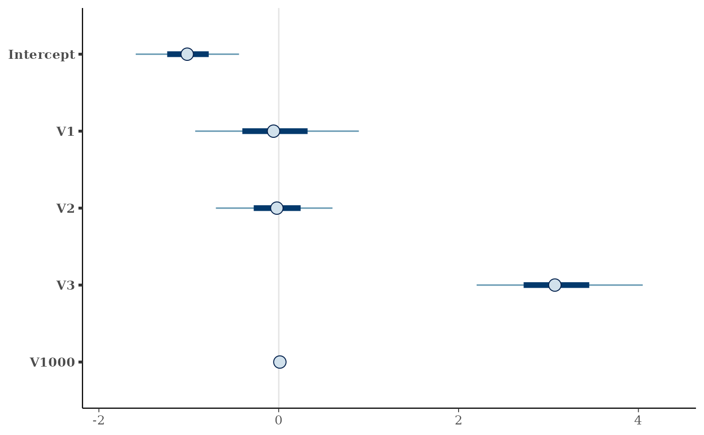
Trace plot of MCMC draws:
as.matrix(fit.t2, k = 2, include.warmup = T) %>%
  mcmc_trace(c("V1", "V1000"), facet_args = list("nrow" = 2), n_warmup = 2000)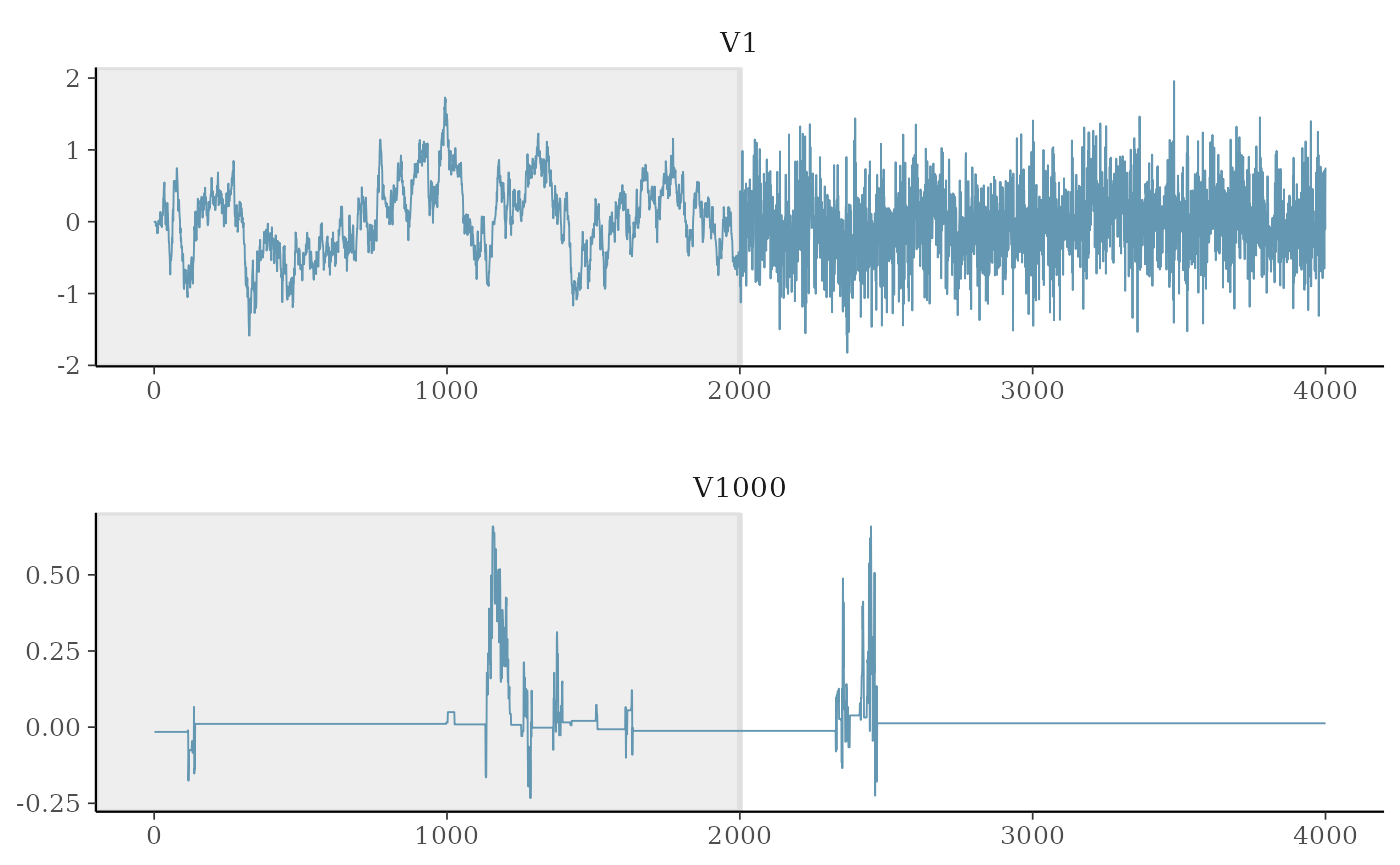
The coefficient of unrelated features (noise) are not updated during some iterations due to restricted Gibbs sampling Li and Yao (2018), hence the computational cost is greatly reduced.
Make Predictions
A glance at the prediction accuracy:
y.class <- predict(fit.t, dat$x.te, type = "class")
y.class
#>       y.pred
#>  [1,]      2
#>  [2,]      2
#>  [3,]      3
#>  [4,]      3
#>  [5,]      2
#>  [6,]      3
#>  [7,]      3
#>  [8,]      2
#>  [9,]      2
#> [10,]      2
print(paste0("prediction accuracy of model 1 = ",
             sum(y.class == dat$y.te) / length(y.class)))
#> [1] "prediction accuracy of model 1 = 0.9"

y.class2 <- predict(fit.t2, dat$x.te, type = "class")
print(paste0("prediction accuracy of model 2 = ",
             sum(y.class2 == dat$y.te) / length(y.class)))
#> [1] "prediction accuracy of model 2 = 0.9"
More details about the prediction result:
predict(fit.t, dat$x.te, type = "response") %>%
  evaluate_pred(y.true = dat$y.te)
#> $prob_at_truelabels
#>  [1] 0.9993980 0.9996598 0.9960531 0.9146809 0.5601952 0.4681349 0.1604013
#>  [8] 0.9999976 0.9986511 0.9655200
#>
#> $table_eval
#>    Case ID True Label Pred. Prob 1 Pred. Prob 2 Pred. Prob 3 Wrong?
#> 1        1          2 2.230163e-04 9.993980e-01 3.789681e-04      0
#> 2        2          2 3.397451e-04 9.996598e-01 4.055238e-07      0
#> 3        3          3 3.946910e-03 3.274933e-09 9.960531e-01      0
#> 4        4          3 8.531913e-02 1.201749e-08 9.146809e-01      0
#> 5        5          2 4.363766e-01 5.601952e-01 3.428135e-03      0
#> 6        6          3 1.231557e-01 4.087093e-01 4.681349e-01      0
#> 7        7          1 1.604013e-01 9.352412e-04 8.386635e-01      1
#> 8        8          2 2.383022e-06 9.999976e-01 3.584158e-08      0
#> 9        9          2 1.339940e-03 9.986511e-01 8.967895e-06      0
#> 10      10          2 3.263762e-02 9.655200e-01 1.842378e-03      0
#>
#> $amlp
#> [1] 0.3299063
#>
#> $err_rate
#> [1] 0.1
#>
#> $which.wrong
#> [1] 7