3  Likelihood Theory

3.1 Definitions and Notations

3.1.1 Regular Families

Definition 3.1 (Regular Families) A family of probability density functions is said to be a Regular Family if the support \(\{\mathbf{x} : f(\mathbf{x}|\boldsymbol{\theta}) > 0\}\) does not depend on the parameter vector \(\boldsymbol{\theta}\).

This condition allows for the interchange of differentiation and integration: \[ \nabla_{\boldsymbol{\theta}} \int \exp\{\ell(\boldsymbol{\theta}; \mathbf{x})\} d\mathbf{x} = \int \nabla_{\boldsymbol{\theta}} \exp\{\ell(\boldsymbol{\theta}; \mathbf{x})\} d\mathbf{x} \]

3.1.2 Score Vector and Fisher Information

Before stating the theorem, we define the following notations for the score and information in the context of a parameter vector \(\boldsymbol{\theta} = (\theta_1, \dots, \theta_p)^T \in \mathbb{R}^p\):

Definition 3.2  

1. Score Vector (\(\mathbf{U}\)): The gradient of the log-likelihood. It is a random column vector of dimension \(p \times 1\). \[ \mathbf{U}(\boldsymbol{\theta}; \mathbf{X}) = \nabla \ell(\boldsymbol{\theta}; \mathbf{X}) = \frac{\partial \ell(\boldsymbol{\theta}; \mathbf{X})}{\partial \boldsymbol{\theta}} = \begin{bmatrix} \frac{\partial \ell(\boldsymbol{\theta}; \mathbf{X})}{\partial \theta_1} \\[6pt] \frac{\partial \ell(\boldsymbol{\theta}; \mathbf{X})}{\partial \theta_2} \\[6pt] \vdots \\[6pt] \frac{\partial \ell(\boldsymbol{\theta}; \mathbf{X})}{\partial \theta_p} \end{bmatrix} \]

2. Observed Information Matrix (\(\mathbf{J}\)): The negative Hessian of the log-likelihood. It is a symmetric random matrix of dimension \(p \times p\), measuring the curvature of the log-likelihood surface. \[ \mathbf{J}(\boldsymbol{\theta}; \mathbf{X}) = - \nabla^2 \ell(\boldsymbol{\theta}; \mathbf{X}) = - \frac{\partial^2 \ell(\boldsymbol{\theta}; \mathbf{X})}{\partial \boldsymbol{\theta} \partial \boldsymbol{\theta}^T} = - \begin{bmatrix} \frac{\partial^2 \ell}{\partial \theta_1^2} & \frac{\partial^2 \ell}{\partial \theta_1 \partial \theta_2} & \cdots & \frac{\partial^2 \ell}{\partial \theta_1 \partial \theta_p} \\[8pt] \frac{\partial^2 \ell}{\partial \theta_2 \partial \theta_1} & \frac{\partial^2 \ell}{\partial \theta_2^2} & \cdots & \frac{\partial^2 \ell}{\partial \theta_2 \partial \theta_p} \\[8pt] \vdots & \vdots & \ddots & \vdots \\[8pt] \frac{\partial^2 \ell}{\partial \theta_p \partial \theta_1} & \frac{\partial^2 \ell}{\partial \theta_p \partial \theta_2} & \cdots & \frac{\partial^2 \ell}{\partial \theta_p^2} \end{bmatrix} \]

3. (Expected) Fisher Information Matrix (\(\mathcal{I}\)): The covariance matrix of the score vector. It is a deterministic \(p \times p\) matrix (for a fixed \(\boldsymbol{\theta}\)). \[ \mathcal{I}(\boldsymbol{\theta}) = E_{\boldsymbol{\theta}} \left[ \mathbf{J}(\boldsymbol{\theta}; \mathbf{X}) \right] \]

3.2 Examples

3.2.1 Exponential Likelihood

Example 3.1 Let \(X_1, \dots, X_n \overset{iid}{\sim} \operatorname{Exp}(\theta)\), where the density is \(f(x|\theta) = \frac{1}{\theta} e^{-x/\theta}\). We use this setting to explore the theoretical connections provided by Bartlett’s Identities and the Cramér-Rao Lower Bound (CRLB).

1. The Score Function (\(U\))

   The Score function is the gradient of the log-likelihood. Bartlett’s first identity suggests that the expected score at the true parameter value is zero, providing the intuition for finding the maximum likelihood estimator (MLE) by setting \(U(\theta) = 0\).

   The log-likelihood function is: \[ \ell(\theta; \mathbf{x}) = \sum_{i=1}^n \left( -\log \theta - \frac{x_i}{\theta} \right) = -n \log \theta - \frac{1}{\theta} \sum_{i=1}^n x_i \]

   The Score function is: \[ U(\theta; \mathbf{x}) = \frac{\partial \ell}{\partial \theta} = -\frac{n}{\theta} + \frac{\sum x_i}{\theta^2} \]

   Bartlett’s First Identity Check: \[E[U] = -\frac{n}{\theta} + \frac{1}{\theta^2} \sum E[X_i] = -\frac{n}{\theta} + \frac{n\theta}{\theta^2} = 0\] (Verified)

2. Fisher Information (\(\mathcal{I}(\theta)\))

   Bartlett’s second identity connects the variance of the Score to the curvature (expected Hessian) of the log-likelihood. This curvature is the Fisher Information.

   • Method A: Negative Expected Hessian \[ U'(\theta) = \frac{\partial U}{\partial \theta} = \frac{n}{\theta^2} - \frac{2\sum x_i}{\theta^3} \] \[ \mathcal{I}(\theta) = -E[U'(\theta)] = -\left( \frac{n}{\theta^2} - \frac{2 n \theta}{\theta^3} \right) = \frac{n}{\theta^2} \]

   • Method B: Variance of the Score \[ \text{Var}(U) = \text{Var}\left( -\frac{n}{\theta} + \frac{\sum X_i}{\theta^2} \right) = \frac{1}{\theta^4} \text{Var}\left( \sum X_i \right) \] Since \(\text{Var}(X_i) = \theta^2\): \[ \text{Var}(U) = \frac{1}{\theta^4} (n \theta^2) = \frac{n}{\theta^2} \]

   Result: \(\text{Var}(U) = \mathcal{I}(\theta)\). (Identity Verified)

3. Cramer-Rao Lower Bound (CRLB)

   The CRLB states that the variance of any unbiased estimator is bounded below by the inverse of the Fisher Information. We test the efficiency of the sample mean \(T(\mathbf{X}) = \bar{X}\).

   • Expectation: \(m(\theta) = E[\bar{X}] = \theta\). Thus, \(T\) is unbiased and \(m'(\theta) = 1\).
   • Actual Variance: \[ \text{Var}(T(\mathbf{X})) = \text{Var}(\bar{X}) = \frac{\text{Var}(X)}{n} = \frac{\theta^2}{n} \]
   • Theoretical Lower Bound: \[ \text{CRLB} = \frac{[m'(\theta)]^2}{\mathcal{I}(\theta)} = \frac{1^2}{n/\theta^2} = \frac{\theta^2}{n} \]

   Conclusion: Since \(\text{Var}(T(\mathbf{X})) = \text{CRLB}\), the estimator \(\bar{X}\) exhausts the information in the sample and is an efficient estimator for \(\theta\).

3.2.2 Cauchy Likelihood (R Illustration)

To illustrate the concepts visually, we use the Cauchy distribution, known for its heavy tails. We assume a known scale of 1 and estimate the location parameter \(\theta\).

The probability density function is \(f(x; \theta) = \frac{1}{\pi (1 + (x-\theta)^2)}\).

The Score Function \(U(\theta)\) is the derivative of the log-likelihood with respect to \(\theta\): \[ U(\theta; \mathbf{x}) = \sum_{i=1}^n \frac{2(x_i - \theta)}{1 + (x_i - \theta)^2} \]

We visualize the Log-Likelihoods (dashed lines) and Score functions (solid lines) for two different sample sizes (\(n=10\) and \(n=20\)) using a true parameter \(\theta^* = 0\).

• Global Scaling: The y-axis ranges are fixed across both plots. Note how the “hills” of the likelihood become sharper and the “slopes” of the score become steeper as \(n\) increases.
• MLE (\(\hat{\theta}\)): The triangles on the x-axis mark the Maximum Likelihood Estimate. Unlike the exponential case, the Cauchy MLE has no closed form and must be found numerically (where the Score crosses zero).
• Score at True Parameter (\(U(\theta^*)\)): The solid circles on the vertical dashed line mark the value of the Score function at the true parameter.

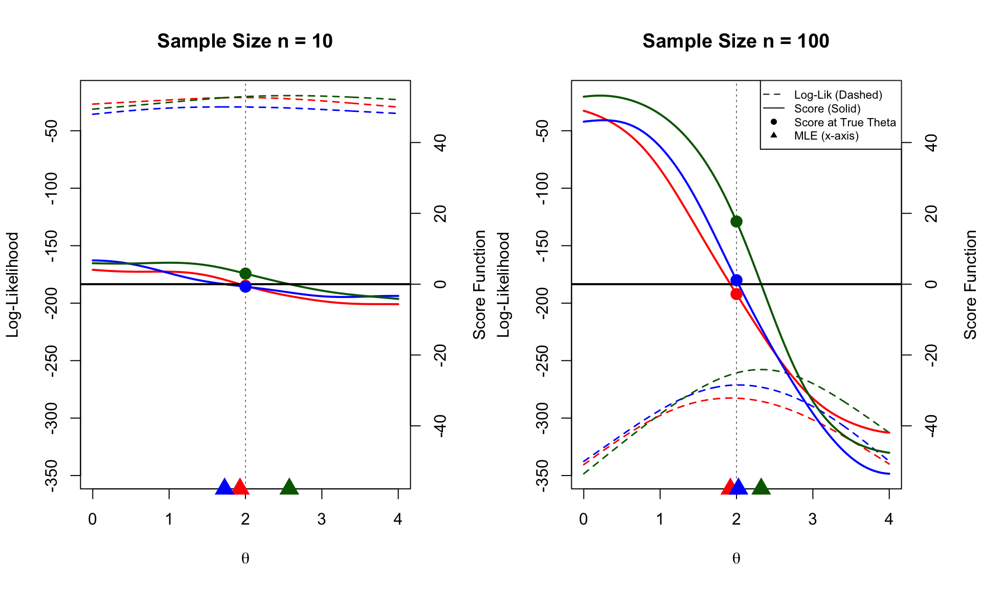
# Parameters
set.seed(1)
theta_true <- 2  # True location parameter
n_sizes <- c(10, 100)
# Grid centered around theta_true
theta_grid <- seq(theta_true-2, theta_true+2, length.out = 300) 

# Define functions for Cauchy (scale=1)
# Log Likelihood: sum( log( 1 / (pi * (1 + (x-theta)^2)) ) )
log_lik_fn <- function(theta, data) {
  sum(dt(data - theta, df = 1, log = TRUE))
}

# Score Function: Gradient of log-likelihood
# d/d_theta [ -log(1 + (x-theta)^2) ] = 2(x-theta) / (1 + (x-theta)^2)
score_fn <- function(theta, data) {
  sum( (2 * (data - theta)) / (1 + (data - theta)^2) )
}

# 1. Generate All Data First
data_list <- list()
for(n in n_sizes) {
  # Generate 3 datasets per sample size (rcauchy)
  data_list[[paste0("n", n)]] <- replicate(3, rcauchy(n, location = theta_true), simplify = FALSE)
}

# 2. Calculate Global Ranges for Consistent Axes
all_lik_vals <- c()
all_score_vals <- c()

for(n_key in names(data_list)) {
  for(d in data_list[[n_key]]) {
    all_lik_vals <- c(all_lik_vals, sapply(theta_grid, log_lik_fn, data=d))
    all_score_vals <- c(all_score_vals, sapply(theta_grid, score_fn, data=d))
  }
}

global_ylim_lik <- range(all_lik_vals)
global_ylim_score <- range(all_score_vals)

# Setup plot layout
par(mfrow = c(1, 2), mar = c(5, 4, 4, 4) + 0.1) 

# Colors for the 3 datasets
cols <- c("red", "blue", "darkgreen")

# 3. Plot Loop
for (n in n_sizes) {
  datasets <- data_list[[paste0("n", n)]]
  
  # --- Plot A: Log-Likelihood (Left Axis) ---
  # NOW DASHED (lty = 2)
  plot(theta_grid, sapply(theta_grid, log_lik_fn, data=datasets[[1]]), 
       type = "l", col = cols[1], lwd = 1.5, lty = 2,
       ylim = global_ylim_lik,  # Global Range
       ylab = "Log-Likelihood", xlab = expression(theta),
       main = paste0("Sample Size n = ", n))
  
  for(i in 2:3){
    lines(theta_grid, sapply(theta_grid, log_lik_fn, data=datasets[[i]]), 
          col = cols[i], lwd = 1.5, lty = 2)
  }
  
  # Mark True Theta Line
  abline(v = theta_true, col = "gray50", lwd = 1, lty=3)

  # --- Plot B: Score Function (Right Axis) ---
  par(new = TRUE)
  
  # NOW SOLID (lty = 1)
  plot(theta_grid, sapply(theta_grid, score_fn, data=datasets[[1]]), 
       type = "l", col = cols[1], lwd = 2, lty = 1, 
       axes = FALSE, xlab = "", ylab = "", 
       ylim = global_ylim_score) # Global Range
  
  for(i in 2:3){
    lines(theta_grid, sapply(theta_grid, score_fn, data=datasets[[i]]), 
          col = cols[i], lwd = 2, lty = 1)
  }
  
  # Right Axis
  axis(4)
  mtext("Score Function", side = 4, line = 3)
  
  # Enhanced U=0 Line
  abline(h = 0, col = "black", lwd = 2) 

  # Marks
  for(i in 1:3){
    # 1. Mark Score at True Theta (Bartlett check)
    sc_val <- score_fn(theta_true, datasets[[i]])
    points(theta_true, sc_val, pch = 19, col = cols[i], cex = 1.5)
    
    # 2. Mark MLE on x-axis (Root finding)
    # Numerical optimization needed for Cauchy MLE
    mle_res <- optimize(f = function(th) log_lik_fn(th, datasets[[i]]), 
                        interval = c(-10, 10), maximum = TRUE)
    mle <- mle_res$maximum
    
    # Place marker at bottom of plot
    points(mle, par("usr")[3], pch = 17, col = cols[i], cex = 2, xpd = TRUE)
  }
  
  # Legend (Only on first plot)
  if (n == n_sizes[2]) { 
     legend("topright", 
            legend = c("Log-Lik (Dashed)", "Score (Solid)", "Score at True Theta", "MLE (x-axis)"),
            lty = c(2, 1, NA, NA), 
            pch = c(NA, NA, 19, 17),
            col = "black", bg="white", cex=0.7)
  }
}

Visualization of the Log-Likelihood, Score Function, MLE of Cauchy Models.

3.3 Bartlett’s Identities: Mean and Covariance of Score Vector

Theorem 3.1 (Bartlett’s Identities: Mean and Covariance of Score Vector) Let \(\{f(\mathbf{x}|\boldsymbol{\theta}) : \boldsymbol{\theta} \in \Theta\}\) be a regular family of probability density functions. The following identities hold relating the moments of the score vector \(\mathbf{U}(\boldsymbol{\theta}; \mathbf{X})\) and the observed information matrix \(\mathbf{J}(\boldsymbol{\theta}; \mathbf{X})\):

1. First Moment Identity: The expected score is zero vector. \[ E_{\boldsymbol{\theta}} [ \mathbf{U}(\boldsymbol{\theta}; \mathbf{X}) ] = \mathbf{0} \]

2. Second Moment Identity: The expected observed information equals to the covariance of the score vector (Fisher Information). \[ \text{Cov}_{\boldsymbol{\theta}} \left( \mathbf{U}(\boldsymbol{\theta}; \mathbf{X}) \right) = E_{\boldsymbol{\theta}} [ \mathbf{J}(\boldsymbol{\theta}; \mathbf{X}) ] = \mathcal{I}(\boldsymbol{\theta}) \]

Remark 3.1. The only assumption in the theorem above is that the families are regular. Therefore, we do not need to assume the log-likelihood \(\ell(\boldsymbol{\theta})\) is “well-behaved” (e.g., approximately quadratic or independence within \(\mathbf{X}\)) for these two identities to hold.

Proof.

1. Proof of the First Moment Identity We start with the fundamental property that a density function integrates to 1 over the sample space of \(\mathbf{X}\): \[ \int f(\mathbf{x}|\boldsymbol{\theta}) \, d\mathbf{x} = 1 \] Differentiating both sides with respect to the parameter vector \(\boldsymbol{\theta}\): \[ \nabla_{\boldsymbol{\theta}} \int f(\mathbf{x}|\boldsymbol{\theta}) \, d\mathbf{x} = \mathbf{0} \] Assuming regularity allows us to interchange differentiation and integration: \[ \int \nabla_{\boldsymbol{\theta}} f(\mathbf{x}|\boldsymbol{\theta}) \, d\mathbf{x} = \mathbf{0} \] Using the identity \(\nabla_{\boldsymbol{\theta}} f(\mathbf{x}|\boldsymbol{\theta}) = f(\mathbf{x}|\boldsymbol{\theta}) \nabla_{\boldsymbol{\theta}} \log f(\mathbf{x}|\boldsymbol{\theta}) = f(\mathbf{x}|\boldsymbol{\theta}) \mathbf{U}(\boldsymbol{\theta}; \mathbf{x})\): \[ \int \mathbf{U}(\boldsymbol{\theta}; \mathbf{x}) f(\mathbf{x}|\boldsymbol{\theta}) \, d\mathbf{x} = \mathbf{0} \] This is precisely the definition of the expectation: \[ E_{\boldsymbol{\theta}} [ \mathbf{U}(\boldsymbol{\theta}; \mathbf{X}) ] = \mathbf{0} \]

2. Proof of the Second Moment Identity We differentiate the result of the First Moment Identity \((E[\mathbf{U}(\boldsymbol{\theta}; \mathbf{X})]=\mathbf{0})\) with respect to \(\boldsymbol{\theta}^T\). \[ \nabla_{\boldsymbol{\theta}^T} \int \mathbf{U}(\boldsymbol{\theta}; \mathbf{x}) f(\mathbf{x}|\boldsymbol{\theta}) \, d\mathbf{x} = \mathbf{0} \] Applying the product rule inside the integral (remembering \(\mathbf{U}\) is a vector): \[ \int \left[ \left( \nabla_{\boldsymbol{\theta}^T} \mathbf{U}(\boldsymbol{\theta}; \mathbf{x}) \right) f(\mathbf{x}|\boldsymbol{\theta}) + \mathbf{U}(\boldsymbol{\theta}; \mathbf{x}) \left( \nabla_{\boldsymbol{\theta}^T} f(\mathbf{x}|\boldsymbol{\theta}) \right) \right] d\mathbf{x} = \mathbf{0} \]

   We analyze the two terms in the bracket:

   • Term 1: \(\nabla_{\boldsymbol{\theta}^T} \mathbf{U}(\boldsymbol{\theta}; \mathbf{x})\) is the Jacobian of the score, which is the Hessian of the log-likelihood, \(\nabla^2 \ell(\boldsymbol{\theta}; \mathbf{x})\). By definition, this is \(-\mathbf{J}(\boldsymbol{\theta}; \mathbf{x})\).
   • Term 2: We use the identity \(\nabla_{\boldsymbol{\theta}^T} f(\mathbf{x}|\boldsymbol{\theta}) = f(\mathbf{x}|\boldsymbol{\theta}) (\nabla_{\boldsymbol{\theta}} \log f(\mathbf{x}|\boldsymbol{\theta}))^T = f(\mathbf{x}|\boldsymbol{\theta}) \mathbf{U}(\boldsymbol{\theta}; \mathbf{x})^T\).

   Substituting these back into the integral: \[ \int \left[ -\mathbf{J}(\boldsymbol{\theta}; \mathbf{x}) f(\mathbf{x}|\boldsymbol{\theta}) + \mathbf{U}(\boldsymbol{\theta}; \mathbf{x}) \mathbf{U}(\boldsymbol{\theta}; \mathbf{x})^T f(\mathbf{x}|\boldsymbol{\theta}) \right] d\mathbf{x} = \mathbf{0} \] This simplifies to expectations: \[ -E_{\boldsymbol{\theta}} [ \mathbf{J}(\boldsymbol{\theta}; \mathbf{X}) ] + E_{\boldsymbol{\theta}} [ \mathbf{U}(\boldsymbol{\theta}; \mathbf{X}) \mathbf{U}(\boldsymbol{\theta}; \mathbf{X})^T ] = \mathbf{0} \] Rearranging gives: \[ E_{\boldsymbol{\theta}} [ \mathbf{J}(\boldsymbol{\theta}; \mathbf{X}) ] = E_{\boldsymbol{\theta}} [ \mathbf{U}(\boldsymbol{\theta}; \mathbf{X}) \mathbf{U}(\boldsymbol{\theta}; \mathbf{X})^T ] \] Finally, recall the definition of the covariance matrix for a random vector with zero mean. Since \(E_{\boldsymbol{\theta}}[\mathbf{U}(\boldsymbol{\theta}; \mathbf{X})] = \mathbf{0}\), we have: \[ \text{Cov}_{\boldsymbol{\theta}}(\mathbf{U}(\boldsymbol{\theta}; \mathbf{X})) = E_{\boldsymbol{\theta}}[\mathbf{U}(\boldsymbol{\theta}; \mathbf{X})\mathbf{U}(\boldsymbol{\theta}; \mathbf{X})^T] - E_{\boldsymbol{\theta}}[\mathbf{U}(\boldsymbol{\theta}; \mathbf{X})]E_{\boldsymbol{\theta}}[\mathbf{U}(\boldsymbol{\theta}; \mathbf{X})]^T = E_{\boldsymbol{\theta}}[\mathbf{U}(\boldsymbol{\theta}; \mathbf{X})\mathbf{U}(\boldsymbol{\theta}; \mathbf{X})^T] \] Therefore, we conclude: \[ \text{Cov}_{\boldsymbol{\theta}}(\mathbf{U}(\boldsymbol{\theta}; \mathbf{X}))=E_{\boldsymbol{\theta}} [ \mathbf{J}(\boldsymbol{\theta}; \mathbf{X}) ] = \mathcal{I}(\boldsymbol{\theta}) \]

3.4 Cramer-Rao Lower Bound

In estimation theory, we often wish to know the limit of how well a parameter can be estimated. The following theorem provides a lower bound on the variance of any estimator.

3.4.1 The Score Covariance Identity

The following theorem establishes a fundamental relationship between the sensitivity of an estimator’s expectation to the parameter \(\boldsymbol{\theta}\) and its covariance with the Score function. This identity is the engine behind the Cramer-Rao Lower Bound.

Theorem 3.2 (Covariance of Estimator and Score) Let \(T(\mathbf{X})\) be any estimator with finite variance, and let \(\mathbf{U}(\boldsymbol{\theta}) = \nabla_{\boldsymbol{\theta}} \log f(\mathbf{X}|\boldsymbol{\theta})\) be the Score function. Under standard regularity conditions, the covariance between the estimator and the score is equal to the derivative of the estimator’s expectation: \[ \text{Cov}_{\boldsymbol{\theta}}(T(\mathbf{X}), \mathbf{U}(\boldsymbol{\theta})) = \nabla_{\boldsymbol{\theta}} E_{\boldsymbol{\theta}}[T(\mathbf{X})] \]

Proof. We evaluate the covariance term explicitly. By definition: \[ \begin{aligned} \text{Cov}_{\boldsymbol{\theta}}(T, \mathbf{U}) &= E_{\boldsymbol{\theta}}[T(\mathbf{X}) \mathbf{U}] - E_{\boldsymbol{\theta}}[T]E_{\boldsymbol{\theta}}[\mathbf{U}] \end{aligned} \] Recall that the expected score is zero (\(E_{\boldsymbol{\theta}}[\mathbf{U}] = \mathbf{0}\)). Thus, the second term vanishes: \[ \begin{aligned} \text{Cov}_{\boldsymbol{\theta}}(T, \mathbf{U}) &= E_{\boldsymbol{\theta}}\left[ T(\mathbf{X}) \nabla_{\boldsymbol{\theta}} \log f(\mathbf{X}|\boldsymbol{\theta}) \right] - m(\boldsymbol{\theta}) \cdot \mathbf{0} \\ &= \int T(\mathbf{x}) \left( \nabla_{\boldsymbol{\theta}} \log f(\mathbf{x}|\boldsymbol{\theta}) \right) f(\mathbf{x}|\boldsymbol{\theta}) \, d\mathbf{x} \end{aligned} \] Using the logarithmic derivative identity \((\nabla_{\boldsymbol{\theta}} \log f) f = \frac{1}{f} (\nabla_{\boldsymbol{\theta}} f) f = \nabla_{\boldsymbol{\theta}} f\): \[ \begin{aligned} \text{Cov}_{\boldsymbol{\theta}}(T, \mathbf{U}) &= \int T(\mathbf{x}) \nabla_{\boldsymbol{\theta}} f(\mathbf{x}|\boldsymbol{\theta}) \, d\mathbf{x} \end{aligned} \] Invoking the regularity condition that allows the interchange of derivative and integral, we move the derivative outside: \[ \text{Cov}_{\boldsymbol{\theta}}(T, \mathbf{U}) = \nabla_{\boldsymbol{\theta}} \int T(\mathbf{x}) f(\mathbf{x}|\boldsymbol{\theta}) \, d\mathbf{x} = \nabla_{\boldsymbol{\theta}} E_{\boldsymbol{\theta}}[T(\mathbf{X})] \] which yields the result: \[ \boxed{\text{Cov}_{\boldsymbol{\theta}}(T, \mathbf{U}) = \nabla m(\boldsymbol{\theta})} \tag{3.1}\]

Theorem 3.3 (Cramer-Rao Lower Bound for Scalar Estimator) Let \(\mathbf{X}\) be a random variable with probability density function (or probability mass function) \(f(\mathbf{x}|\boldsymbol{\theta})\), where \(\boldsymbol{\theta} \in \Theta\) is a vector unknown parameter. Let \(T(\mathbf{X})\) be any estimator with finite variance, and let \(m(\boldsymbol{\theta}) = E_{\boldsymbol{\theta}}[T(\mathbf{X})]\) denote its expectation.

Assume the following regularity conditions hold:

1. The support of \(\mathbf{X}\), denoted \(\mathcal{X} = \{\mathbf{x} : f(\mathbf{x}|\boldsymbol{\theta}) > 0\}\), does not depend on \(\boldsymbol{\theta}\).
2. The differentiation with respect to \(\boldsymbol{\theta}\) and integration (or summation) with respect to \(\mathbf{x}\) can be interchanged.

Then, the variance of \(T(\mathbf{X})\) satisfies: \[ \text{Var}_{\boldsymbol{\theta}}(T(\mathbf{X})) \ge \frac{[\nabla m(\boldsymbol{\theta})]^2}{\mathcal{I}(\boldsymbol{\theta})} \] where \(\mathcal{I}(\boldsymbol{\theta}) = E_{\boldsymbol{\theta}} \left[ \left( \nabla_{\boldsymbol{\theta}} \log f(\mathbf{X}|\boldsymbol{\theta}) \right)^2 \right]\) is the Fisher Information.

Particular Case: If \(T(\mathbf{X})\) is an unbiased estimator of \(\boldsymbol{\theta}\) (i.e., \(m(\boldsymbol{\theta}) = \boldsymbol{\theta}\) and \(\nabla m(\boldsymbol{\theta})=\mathbf{I}\)), then: \[ \text{Var}_{\boldsymbol{\theta}}(T(\mathbf{X})) \ge \frac{1}{\mathcal{I}(\boldsymbol{\theta})} \]

Proof. Let \(\mathbf{U} = \nabla_{\boldsymbol{\theta}} \log f(\mathbf{X}|\boldsymbol{\theta})\) be the Score function. From the properties of the Score function under the stated regularity conditions, we know that the score has mean zero and variance equal to the Fisher Information: \[ E_{\boldsymbol{\theta}}[\mathbf{U}] = \mathbf{0} \quad \text{and} \quad \text{Var}_{\boldsymbol{\theta}}(\mathbf{U}) = \mathcal{I}(\boldsymbol{\theta}) \] Consider the covariance between the estimator \(T(\mathbf{X})\) and the Score \(\mathbf{U}\). By the Cauchy-Schwarz inequality: \[ [\text{Cov}_{\boldsymbol{\theta}}(T, \mathbf{U})]^2 \le \text{Var}_{\boldsymbol{\theta}}(T) \text{Var}_{\boldsymbol{\theta}}(\mathbf{U}) \] Using the Score Covariance Identity (Theorem 3.2), we substitute the explicit form of the covariance: \[ \text{Cov}_{\boldsymbol{\theta}}(T, \mathbf{U}) = \nabla m(\boldsymbol{\theta}) \] Substituting this result and \(\text{Var}_{\boldsymbol{\theta}}(\mathbf{U}) = \mathcal{I}(\boldsymbol{\theta})\) back into the covariance inequality: \[ [\nabla m(\boldsymbol{\theta})]^2 \le \text{Var}_{\boldsymbol{\theta}}(T) \cdot \mathcal{I}(\boldsymbol{\theta}) \] Rearranging the terms yields the desired lower bound: \[ \text{Var}_{\boldsymbol{\theta}}(T(\mathbf{X})) \ge \frac{[\nabla m(\boldsymbol{\theta})]^2}{\mathcal{I}(\boldsymbol{\theta})} \]

Figure 3.1 illustrates the relationship between the curvature of the log-likelihood (Fisher Information) and the variance of the estimator. A sharper peak implies higher information and lower variance.

Figure 3.1: Fisher Information: Curvature vs. Variance

Remark 3.2 (Generality of the Lower Bound). The power of the Cramer-Rao Lower Bound lies in its independence from the specific method of estimation. It relies solely on the properties of the underlying probability model (specifically, the curvature of the log-likelihood function) and the bias of the estimator. Consequently, it provides a universal benchmark for precision:

1. Fundamental Limit: It represents the limit of “extractable information” about \(\boldsymbol{\theta}\) contained in the data \(\mathbf{X}\). No matter how clever the estimation algorithm is (e.g., Method of Moments, Bayes estimators, etc.), the variance cannot be reduced beyond this intrinsic bound determined by the Fisher Information.
2. Efficiency Standard: It allows us to define the concept of an efficient estimator. Any unbiased estimator that attains this lower bound is the Uniformly Minimum Variance Unbiased Estimator (UMVUE).
3. Asymptotic Justification: While finite-sample estimators may not always achieve this bound, the Maximum Likelihood Estimator (MLE) is asymptotically efficient. This means that as the sample size \(n \to \infty\), the variance of the MLE approaches the CRLB, justifying the popularity of likelihood-based inference.

3.4.2 Multivariate Cramer-Rao Lower Bound

Theorem 3.4 (Multivariate Cramer-Rao Lower Bound) Let \(\mathbf{X}\) be a random vector with density \(f(\mathbf{x}|\boldsymbol{\theta})\), where \(\boldsymbol{\theta} \in \mathbb{R}^p\) is a vector of unknown parameters. Let \(\mathbf{T}(\mathbf{X}) \in \mathbb{R}^k\) be any estimator with finite covariance matrix, and let \(\mathbf{m}(\boldsymbol{\theta}) = E_{\boldsymbol{\theta}}[\mathbf{T}(\mathbf{X})]\) denote its expectation vector.

Let \(\mathcal{I}(\boldsymbol{\theta})\) be the \(p \times p\) Fisher Information Matrix: \[ \mathcal{I}(\boldsymbol{\theta}) = E_{\boldsymbol{\theta}} \left[ \mathbf{U}(\boldsymbol{\theta}; \mathbf{X}) \mathbf{U}(\boldsymbol{\theta}; \mathbf{X})^\top \right] \] Let \(\mathbf{D}(\boldsymbol{\theta}) = \frac{\partial \mathbf{m}(\boldsymbol{\theta})}{\partial \boldsymbol{\theta}}\) be the \(k \times p\) Jacobian matrix of the expectation, where \(D_{ij} = \frac{\partial m_i}{\partial \theta_j}\).

Under standard regularity conditions, the covariance matrix of \(\mathbf{T}\) satisfies the inequality: \[ \text{Var}_{\boldsymbol{\theta}}(\mathbf{T}) \succeq \mathbf{D}(\boldsymbol{\theta}) [\mathcal{I}(\boldsymbol{\theta})]^{-1} \mathbf{D}(\boldsymbol{\theta})^\top \] Here, \(\mathbf{A} \succeq \mathbf{B}\) means that the matrix \(\mathbf{A} - \mathbf{B}\) is positive semi-definite.

Proof. Let \(\mathbf{U} = \nabla_{\boldsymbol{\theta}} \log f(\mathbf{X}|\boldsymbol{\theta})\) be the \(p \times 1\) Score vector. We know that \(E[\mathbf{U}] = \mathbf{0}\) and \(\text{Var}(\mathbf{U}) = \mathcal{I}(\boldsymbol{\theta})\).

We apply the multivariate extension of the Score Covariance Identity (Theorem 3.2). This identity states that the covariance between an estimator and the score vector is the Jacobian of the estimator’s expectation: \[ \text{Cov}(\mathbf{T}, \mathbf{U}) = E[\mathbf{T} \mathbf{U}^\top] = \mathbf{D}(\boldsymbol{\theta}) \]

Now, define the block vector \(\mathbf{Z} = \begin{pmatrix} \mathbf{T} \\ \mathbf{U} \end{pmatrix}\). The covariance matrix of \(\mathbf{Z}\) is necessarily positive semi-definite: \[ \text{Var}(\mathbf{Z}) = \begin{pmatrix} \text{Var}(\mathbf{T}) & \text{Cov}(\mathbf{T}, \mathbf{U}) \\ \text{Cov}(\mathbf{U}, \mathbf{T}) & \text{Var}(\mathbf{U}) \end{pmatrix} = \begin{pmatrix} \Sigma_{\mathbf{T}} & \mathbf{D} \\ \mathbf{D}^\top & \mathcal{I} \end{pmatrix} \succeq 0 \]

For this block matrix to be positive semi-definite, the Schur complement of the block \(\mathcal{I}\) must be positive semi-definite (assuming \(\mathcal{I}\) is positive definite/invertible): \[ \Sigma_{\mathbf{T}} - \mathbf{D} \mathcal{I}^{-1} \mathbf{D}^\top \succeq 0 \]

Thus, we obtain the bound: \[ \text{Var}(\mathbf{T}) \succeq \mathbf{D} \mathcal{I}^{-1} \mathbf{D}^\top \]

3.4.3 Connection to Stein’s Lemma

The Score Covariance Identity (\(\text{Cov}(\mathbf{T}, \mathbf{U}) = \mathbf{D}(\boldsymbol{\theta})\)) derived in the proof of the CRLB is a fundamental result that links the sensitivity of an estimator to its correlation with the score. When applied to the Normal distribution, this identity specializes to the famous Stein’s Lemma, which relates the covariance of a function and the random vector to the expected gradient of the function.

Theorem 3.5 (Stein’s Lemma for Scalar \(g(\mathbf{X})\)) Let \(\mathbf{X} \sim \mathcal{N}(\boldsymbol{\theta}, \sigma^2 \mathbf{I})\), where \(\boldsymbol{\theta} \in \mathbb{R}^p\) is the mean vector and \(\sigma^2 > 0\) is a known scalar variance. Let \(g: \mathbb{R}^p \to \mathbb{R}\) be a differentiable function such that \(E[\|\nabla g(\mathbf{X})\|] < \infty\).

Then, the following identity holds: \[ \text{Cov}(g(\mathbf{X}), \mathbf{X}) = \sigma^2 E[\nabla g(\mathbf{X})] \] where \(\nabla g(\mathbf{X})\) is the gradient vector of \(g\) with respect to \(\mathbf{X}\).

Proof. Proof via Score Covariance Identity

1. The Score Function: For \(\mathbf{X} \sim \mathcal{N}(\boldsymbol{\theta}, \sigma^2 \mathbf{I})\), the log-likelihood is quadratic, and the score vector is linear in \(\mathbf{X}\): \[ \mathbf{U}(\boldsymbol{\theta}) = \nabla_{\boldsymbol{\theta}} \log f(\mathbf{x}|\boldsymbol{\theta}) = \frac{1}{\sigma^2}(\mathbf{X} - \boldsymbol{\theta}) \]

2. Applying the Score Covariance Identity: From the proof of the CRLB, we established the identity \(\text{Cov}(T, \mathbf{U}) = \nabla_{\boldsymbol{\theta}} E[T]\) for any statistic \(T\). Letting \(T = g(\mathbf{X})\), we substitute the Normal score \(\mathbf{U}\): \[ \text{Cov}\left( g(\mathbf{X}), \frac{\mathbf{X} - \boldsymbol{\theta}}{\sigma^2} \right) = \nabla_{\boldsymbol{\theta}} E_{\boldsymbol{\theta}}[g(\mathbf{X})] \] Using the linearity of covariance, the Left-Hand Side (LHS) simplifies to: \[ \text{LHS} = \frac{1}{\sigma^2} \text{Cov}(g(\mathbf{X}), \mathbf{X}) \]

3. Evaluating the Sensitivity (RHS): We evaluate the sensitivity of the expectation \(\nabla_{\boldsymbol{\theta}} E_{\boldsymbol{\theta}}[g(\mathbf{X})]\). Using the substitution \(\mathbf{z} = \mathbf{x} - \boldsymbol{\theta}\) (which removes \(\boldsymbol{\theta}\) from the density \(f\) and puts it into \(g\)): \[ E_{\boldsymbol{\theta}}[g(\mathbf{X})] = \int g(\mathbf{z} + \boldsymbol{\theta}) f(\mathbf{z}) \, d\mathbf{z} \] Differentiating with respect to \(\boldsymbol{\theta}\) and noting that \(\nabla_{\boldsymbol{\theta}} g(\mathbf{z} + \boldsymbol{\theta}) = \nabla_{\mathbf{x}} g(\mathbf{x})\): \[ \nabla_{\boldsymbol{\theta}} E_{\boldsymbol{\theta}}[g(\mathbf{X})] = \int \nabla g(\mathbf{z} + \boldsymbol{\theta}) f(\mathbf{z}) \, d\mathbf{z} = E[\nabla g(\mathbf{X})] \]

4. Conclusion: Equating the LHS and RHS: \[ \frac{1}{\sigma^2} \text{Cov}(g(\mathbf{X}), \mathbf{X}) = E[\nabla g(\mathbf{X})] \] Multiplying by \(\sigma^2\) yields the result.

3.4.4 Stein’s Lemma (Multivariate Divergence Form)

Let \(\mathbf{X} \sim \mathcal{N}(\boldsymbol{\theta}, \sigma^2 \mathbf{I})\), where \(\boldsymbol{\theta} \in \mathbb{R}^p\) is the mean vector and \(\sigma^2 > 0\) is a known scalar variance. Let \(\mathbf{g}: \mathbb{R}^p \to \mathbb{R}^p\) be a differentiable vector-valued function, denoted \(\mathbf{g}(\mathbf{x}) = (g_1(\mathbf{x}), \dots, g_p(\mathbf{x}))^\top\), such that \(E[| \nabla \cdot \mathbf{g}(\mathbf{X}) |] < \infty\).

Then, the following identity holds: \[ E \left[ (\mathbf{X} - \boldsymbol{\theta})^\top \mathbf{g}(\mathbf{X}) \right] = \sigma^2 E \left[ \nabla \cdot \mathbf{g}(\mathbf{X}) \right] \] where \(\nabla \cdot \mathbf{g}(\mathbf{X}) = \sum_{i=1}^p \frac{\partial g_i}{\partial x_i}\) is the divergence of \(\mathbf{g}\).

Proof. Proof via Component-wise Score Identity

1. The Score Function: The score vector for the Normal distribution is \(\mathbf{U}(\boldsymbol{\theta}) = \frac{1}{\sigma^2}(\mathbf{X} - \boldsymbol{\theta})\).
2. Applying the Scalar Identity Component-wise: Let’s look at the \(i\)-th component of the vector function, \(g_i(\mathbf{X})\). Treating \(g_i\) as a scalar estimator and \(X_i\) as the data, we apply the scalar score identity (or simply integration by parts on the \(i\)-th coordinate): \[ \text{Cov}(g_i(\mathbf{X}), X_i) = \sigma^2 E \left[ \frac{\partial g_i(\mathbf{X})}{\partial x_i} \right] \] Note that \(\text{Cov}(g_i(\mathbf{X}), X_i) = E[(X_i - \theta_i) g_i(\mathbf{X})]\).
3. Summing Components: We sum the identity over all \(p\) dimensions: \[ \sum_{i=1}^p E \left[ (X_i - \theta_i) g_i(\mathbf{X}) \right] = \sigma^2 \sum_{i=1}^p E \left[ \frac{\partial g_i(\mathbf{X})}{\partial x_i} \right] \]
4. Vector Notation: The Left-Hand Side is the expected inner product \(E[(\mathbf{X} - \boldsymbol{\theta})^\top \mathbf{g}(\mathbf{X})]\). The Right-Hand Side is the scaled expected divergence \(\sigma^2 E[\nabla \cdot \mathbf{g}(\mathbf{X})]\). \[ E \left[ (\mathbf{X} - \boldsymbol{\theta})^\top \mathbf{g}(\mathbf{X}) \right] = \sigma^2 E \left[ \nabla \cdot \mathbf{g}(\mathbf{X}) \right] \]

NoteSignificance: Stein’s Unbiased Risk Estimate (SURE)

This divergence form is famous for enabling SURE. If we estimate \(\boldsymbol{\theta}\) using \(\hat{\boldsymbol{\theta}} = \mathbf{X} + \mathbf{g}(\mathbf{X})\), we can estimate the Mean Squared Error (MSE) purely from the data, because Stein’s Lemma allows us to replace the unknown cross-term involving \(\boldsymbol{\theta}\) with the observable divergence \(\nabla \cdot \mathbf{g}(\mathbf{X}).\)

3.5 Differentiated Log Likelihood

3.5.1 Mean and Covariance of Score Vector \(U(\boldsymbol{\theta};\mathbf{X})\).

We can also establish Bartlett’s identities by analyzing the properties of the likelihood ratio expectation.

Proof. Let \(\mathbf{X}\) be a random vector with density \(f(\mathbf{x}|\boldsymbol{\theta})\). We define the function \(M(\mathbf{t})\) as the expected value of the likelihood ratio between parameters \(\boldsymbol{\theta}+\mathbf{t}\) and \(\boldsymbol{\theta}\), where \(\mathbf{t}\) is a perturbation vector. \[ M(\mathbf{t}) = E_{\boldsymbol{\theta}} \left[ \exp\left( \ell(\boldsymbol{\theta} + \mathbf{t; X}) - \ell(\boldsymbol{\theta; X}) \right) \right] \] Since \(E_{\boldsymbol{\theta}} \left[ \frac{f(\mathbf{X}|\boldsymbol{\theta}+\mathbf{t})}{f(\mathbf{X}|\boldsymbol{\theta})} \right] = \int f(\mathbf{x}|\boldsymbol{\theta}+\mathbf{t}) \, d\mathbf{x} = 1\), we have the identity: \[ M(\mathbf{t}) \equiv 1 \quad \text{for all } \mathbf{t} \] We expand the log-likelihood difference \(\Delta \ell(\mathbf{t}) = \ell(\boldsymbol{\theta} + \mathbf{t}) - \ell(\boldsymbol{\theta})\) using a Taylor series around \(\mathbf{t} = \mathbf{0}\): \[ \Delta \ell(\mathbf{t}) = \mathbf{U}(\boldsymbol{\theta})^T \mathbf{t} - \frac{1}{2} \mathbf{t}^T \mathbf{J}(\boldsymbol{\theta}) \mathbf{t} + o(\|\mathbf{t}\|^2) \] Substituting this into \(M(\mathbf{t})\) and expanding the exponential function: \[ \begin{aligned} M(\mathbf{t}) &= E_{\boldsymbol{\theta}} \left[ \exp\left( \mathbf{U}^T \mathbf{t} - \frac{1}{2} \mathbf{t}^T \mathbf{J} \mathbf{t} + o(\|\mathbf{t}\|^2) \right) \right] \\ &= E_{\boldsymbol{\theta}} \left[ 1 + \left( \mathbf{U}^T \mathbf{t} - \frac{1}{2} \mathbf{t}^T \mathbf{J} \mathbf{t} \right) + \frac{1}{2} \left( \mathbf{U}^T \mathbf{t} \right)^2 + o(\|\mathbf{t}\|^2) \right] \\ &= 1 + \mathbf{t}^T E_{\boldsymbol{\theta}}[\mathbf{U}] + \frac{1}{2} \mathbf{t}^T \left( E_{\boldsymbol{\theta}}[\mathbf{U}\mathbf{U}^T] - E_{\boldsymbol{\theta}}[\mathbf{J}] \right) \mathbf{t} + o(\|\mathbf{t}\|^2) \end{aligned} \] Since \(M(\mathbf{t}) \equiv 1\), the coefficients of the linear and quadratic terms in \(\mathbf{t}\) must be zero:

1. Linear Term: \(\mathbf{t}^T E_{\boldsymbol{\theta}}[\mathbf{U}] = 0 \implies E_{\boldsymbol{\theta}}[\mathbf{U}] = \mathbf{0}\).
2. Quadratic Term: \(E_{\boldsymbol{\theta}}[\mathbf{U}\mathbf{U}^T] - E_{\boldsymbol{\theta}}[\mathbf{J}] = \mathbf{0} \implies \text{Cov}(\mathbf{U}) = E_{\boldsymbol{\theta}}[\mathbf{J}]\).

3.5.2 Alternative Proof of CRLB

We can prove the CRLB using the likelihood ratio expansion method. This approach relates the sensitivity of the estimator (the derivative of its expectation) to its correlation with the score function.

Proof.

1. Setup the Perturbed Expectation: Consider the expectation of the estimator \(\mathbf{T}(\mathbf{X})\) under a slightly shifted parameter \(\boldsymbol{\theta} + \mathbf{t}\). We can express this as an expectation under the original parameter \(\boldsymbol{\theta}\) using the likelihood ratio: \[ \mathbf{m}(\boldsymbol{\theta} + \mathbf{t}) = E_{\boldsymbol{\theta} + \mathbf{t}}[\mathbf{T}(\mathbf{X})] = E_{\boldsymbol{\theta}} \left[ \mathbf{T}(\mathbf{X}) \frac{f(\mathbf{X}|\boldsymbol{\theta} + \mathbf{t})}{f(\mathbf{X}|\boldsymbol{\theta})} \right] \] This can be written using the log-likelihood difference \(\Delta \ell = \ell(\boldsymbol{\theta} + \mathbf{t}) - \ell(\boldsymbol{\theta})\): \[ \mathbf{m}(\boldsymbol{\theta} + \mathbf{t}) = E_{\boldsymbol{\theta}} \left[ \mathbf{T}(\mathbf{X}) \exp(\Delta \ell) \right] \]

2. Taylor Expansion (Left Side): We expand the expectation vector \(\mathbf{m}(\boldsymbol{\theta} + \mathbf{t})\) around \(\mathbf{t}=\mathbf{0}\). By definition, the linear term is the Jacobian matrix \(\mathbf{D}(\boldsymbol{\theta}) = \frac{\partial \mathbf{m}}{\partial \boldsymbol{\theta}}\): \[ \mathbf{m}(\boldsymbol{\theta} + \mathbf{t}) = \mathbf{m}(\boldsymbol{\theta}) + \mathbf{D}(\boldsymbol{\theta}) \mathbf{t} + o(\|\mathbf{t}\|) \]

3. Taylor Expansion (Right Side): We expand the likelihood ratio term \(\exp(\Delta \ell)\). Since \(\Delta \ell \approx \mathbf{U}(\boldsymbol{\theta})^T \mathbf{t}\), we have \(\exp(\Delta \ell) \approx 1 + \mathbf{U}(\boldsymbol{\theta})^T \mathbf{t}\). \[ \begin{aligned} E_{\boldsymbol{\theta}} \left[ \mathbf{T}(\mathbf{X}) (1 + \mathbf{U}^T \mathbf{t} + \dots) \right] &= E_{\boldsymbol{\theta}}[\mathbf{T}] + E_{\boldsymbol{\theta}}[\mathbf{T} \mathbf{U}^T \mathbf{t}] + \dots \\ &= \mathbf{m}(\boldsymbol{\theta}) + E_{\boldsymbol{\theta}}[\mathbf{T} \mathbf{U}^T] \mathbf{t} + o(\|\mathbf{t}\|) \end{aligned} \]

4. Matching Linear Coefficients: Since the Left Side must equal the Right Side for any perturbation \(\mathbf{t}\), the coefficients of the linear term \(\mathbf{t}\) must be identical: \[ \mathbf{D}(\boldsymbol{\theta}) = E_{\boldsymbol{\theta}}[\mathbf{T} \mathbf{U}^T] \]

5. Linking to Covariance: Recall that the score vector has mean zero, \(E[\mathbf{U}] = \mathbf{0}\). Therefore, the term \(E[\mathbf{T} \mathbf{U}^T]\) is exactly the covariance between the estimator and the score: \[ \text{Cov}(\mathbf{T}, \mathbf{U}) = E[\mathbf{T} \mathbf{U}^T] - E[\mathbf{T}]\underbrace{E[\mathbf{U}]^T}_{\mathbf{0}} = E[\mathbf{T} \mathbf{U}^T] \] Thus, we have the crucial identity: \[ \mathbf{D}(\boldsymbol{\theta}) = \text{Cov}(\mathbf{T}, \mathbf{U}) \]

6. Deriving the Inequality: To obtain the bound, we construct the joint covariance matrix of the vector \(\mathbf{Z} = \begin{pmatrix} \mathbf{T} \\ \mathbf{U} \end{pmatrix}\). This matrix must be positive semi-definite (PSD). \[ \text{Var}\begin{pmatrix} \mathbf{T} \\ \mathbf{U} \end{pmatrix} = \begin{pmatrix} \text{Var}(\mathbf{T}) & \text{Cov}(\mathbf{T}, \mathbf{U}) \\ \text{Cov}(\mathbf{U}, \mathbf{T}) & \text{Var}(\mathbf{U}) \end{pmatrix} = \begin{pmatrix} \Sigma_\mathbf{T} & \mathbf{D} \\ \mathbf{D}^T & \mathcal{I} \end{pmatrix} \succeq 0 \] By the property of Schur complements, for a block matrix to be PSD, the complement of the bottom-right block must be PSD: \[ \Sigma_\mathbf{T} - \mathbf{D} \mathcal{I}^{-1} \mathbf{D}^T \succeq 0 \] Rearranging this gives the Multivariate Cramer-Rao Lower Bound: \[ \text{Var}(\mathbf{T}) \succeq \mathbf{D}(\boldsymbol{\theta}) [\mathcal{I}(\boldsymbol{\theta})]^{-1} \mathbf{D}(\boldsymbol{\theta})^T \]

3.6 Exponential Families

A family of probability distributions is defined by the specific mathematical way the parameters and the data interact. For most common distributions, this interaction can be factored into a form that simplifies both theoretical analysis and computational estimation.

Definition 3.3 (Exponential Family) A family of probability density functions (or mass functions) \(\{f(\mathbf{x}|\boldsymbol{\theta}) : \boldsymbol{\theta} \in \Theta\}\) is called a \(k\)-parameter Exponential Family if it can be expressed in the following equivalent forms:

1. Density Form The probability density function is written as:

   \[ f(\mathbf{x}|\boldsymbol{\theta}) = h(\mathbf{x}) \exp \left( \sum_{i=1}^k \eta_i(\boldsymbol{\theta}) T_i(\mathbf{x}) - A(\boldsymbol{\theta}) \right) \]

2. Log-Likelihood Form By taking the natural logarithm, the log-likelihood for a single observation (or a joint sample) is:

   \[ \ell(\boldsymbol{\theta}; \mathbf{x}) = \sum_{i=1}^k \eta_i(\boldsymbol{\theta}) T_i(\mathbf{x}) - A(\boldsymbol{\theta}) + \log h(\mathbf{x}) \]

where the components are defined as:

1. \(h(\mathbf{x}) \ge 0\) The base measure, which is a function depending only on the data \(\mathbf{x}\) and not on the parameter \(\boldsymbol{\theta}\).

2. \(T_i(\mathbf{x})\) The components of the sufficient statistic vector \(\mathbf{T}(\mathbf{x}) = (T_1(\mathbf{x}), \dots, T_k(\mathbf{x}))^T\).

3. \(\eta_i(\boldsymbol{\theta})\) The natural parameters (or canonical parameters) which determine how the sufficient statistics contribute to the likelihood.

4. \(A(\boldsymbol{\theta})\) The log-partition function (or cumulant function). It is a normalization constant that ensures the density integrates to 1, defined by:

   \[ A(\boldsymbol{\theta}) = \log \left( \int h(\mathbf{x}) \exp \left( \sum_{i=1}^k \eta_i(\boldsymbol{\theta}) T_i(\mathbf{x}) \right) d\mathbf{x} \right) \]

3.6.1 Examples

Exponential Distribution

Example 3.2 (Exponential Distribution) Let \(X_1, \dots, X_n \overset{iid}{\sim} \text{Exp}(\theta)\), where \(\theta\) is the scale parameter. \[ f(\mathbf{x}|\theta) = \theta^{-n} \exp\left\{ -\frac{1}{\theta} \sum_{i=1}^n x_i \right\} \]

The log-likelihood is: \[ \ell(\theta; \mathbf{x}) = -\frac{1}{\theta} \sum_{i=1}^n x_i - n \log \theta \]

Identifying the components: - \(\eta_1(\theta) = -\frac{1}{\theta}\) - \(T_1(\mathbf{x}) = \sum_{i=1}^n x_i\) - \(A(\theta) = n \log \theta\) - \(\log h(\mathbf{x}) = 0\)

Gamma Distribution

Example 3.3 (Gamma Distribution) Let \(X_1, \dots, X_n \overset{iid}{\sim} \text{Gamma}(\alpha, \beta)\). The density is: \[ f(\mathbf{x}|\boldsymbol{\theta}) = [\Gamma(\alpha)\beta^\alpha]^{-n} \left( \prod_{i=1}^n x_i \right)^{\alpha-1} \exp\left\{ -\frac{1}{\beta} \sum_{i=1}^n x_i \right\} \]

The log-likelihood is: \[ \ell(\boldsymbol{\theta}; \mathbf{x}) = (\alpha-1) \sum_{i=1}^n \log x_i - \frac{1}{\beta} \sum_{i=1}^n x_i - \left[ n \log \Gamma(\alpha) + n\alpha \log \beta \right] \]

Identifying the components: - \(\eta_1(\boldsymbol{\theta}) = \alpha - 1, \quad T_1(\mathbf{x}) = \sum \log x_i\) - \(\eta_2(\boldsymbol{\theta}) = -\frac{1}{\beta}, \quad T_2(\mathbf{x}) = \sum x_i\) - \(A(\boldsymbol{\theta}) = n \log \Gamma(\alpha) + n\alpha \log \beta\)

Beta Distribution

Example 3.4 (Beta Distribution) Let \(X_1, \dots, X_n \overset{iid}{\sim} \text{Beta}(a, b)\) with \(\boldsymbol{\theta} = (a, b)\). \[ \ell(\boldsymbol{\theta}; \mathbf{x}) = (a-1) \sum_{i=1}^n \log x_i + (b-1) \sum_{i=1}^n \log(1-x_i) - n \log B(a, b) \]

This is an exponential family with \(k=2\). - \(\eta_1 = a-1\), \(T_1 = \sum \log x_i\) - \(\eta_2 = b-1\), \(T_2 = \sum \log(1-x_i)\) - \(A(\boldsymbol{\theta}) = n \log B(a, b)\)

Normal Distribution

Example 3.5 (Normal Distribution) Let \(X_1, \dots, X_n \overset{iid}{\sim} N(\mu, \sigma^2)\). The log-likelihood is: \[ \ell(\boldsymbol{\theta}; \mathbf{x}) = \frac{\mu}{\sigma^2} \sum_{i=1}^n x_i - \frac{1}{2\sigma^2} \sum_{i=1}^n x_i^2 - \left[ \frac{n\mu^2}{2\sigma^2} + \frac{n}{2} \log(2\pi\sigma^2) \right] \]

Identifying the components: - \(\eta_1 = \frac{\mu}{\sigma^2}\), \(T_1 = \sum x_i\) - \(\eta_2 = -\frac{1}{2\sigma^2}\), \(T_2 = \sum x_i^2\) - \(A(\boldsymbol{\theta}) = \frac{n\mu^2}{2\sigma^2} + n \log \sigma + \frac{n}{2} \log(2\pi)\)

3.6.2 Examples of Non-exponential Families

A model is not in the exponential family if the support depends on the parameter.

Uniform Distribution

Example 3.6 (Uniform Distribution) Let \(X \sim U(0, \theta)\). \[ \ell(\theta; x) = -\log \theta + \log I(0 < x < \theta) \] The term \(\log I(0 < x < \theta)\) couples \(x\) and \(\theta\) in a way that cannot be separated into a sum \(\sum \eta_i(\theta) T_i(x).\)

3.6.3 Moments of Sufficient Statistics of Exponential Families

3.6.3.1 Means of Sufficient Statistics (General Case)

Theorem 3.6 (Means via the Score Function) For a regular exponential family with log-likelihood \(\ell(\boldsymbol{\theta}; \mathbf{x}) = \sum \eta_i(\boldsymbol{\theta}) T_i(\mathbf{x}) - A(\boldsymbol{\theta}) + \log h(\mathbf{x})\), the expectation of the sufficient statistics can be found by setting the expected score to zero: \[ E_{\boldsymbol{\theta}} \left[ \frac{\partial \ell(\boldsymbol{\theta}; \mathbf{X})}{\partial \theta_j} \right] = 0 \]

Substituting the specific form of \(\ell(\boldsymbol{\theta}; \mathbf{X})\): \[ \sum_{i=1}^k \frac{\partial \eta_i(\boldsymbol{\theta})}{\partial \theta_j} E[T_i(\mathbf{X})] = \frac{\partial A(\boldsymbol{\theta})}{\partial \theta_j} \quad \text{for } j=1, \dots, d \]

Proof. The log-likelihood is: \[ \ell(\boldsymbol{\theta}; \mathbf{x}) = \sum_{i=1}^k \eta_i(\boldsymbol{\theta}) T_i(\mathbf{x}) - A(\boldsymbol{\theta}) + \log h(\mathbf{x}) \] Differentiating with respect to \(\theta_j\): \[ \frac{\partial \ell}{\partial \theta_j} = \sum_{i=1}^k \frac{\partial \eta_i(\boldsymbol{\theta})}{\partial \theta_j} T_i(\mathbf{x}) - \frac{\partial A(\boldsymbol{\theta})}{\partial \theta_j} \] Taking the expectation and using the regularity condition \(E[\frac{\partial \ell}{\partial \theta_j}] = 0\): \[ E\left[ \sum_{i=1}^k \frac{\partial \eta_i(\boldsymbol{\theta})}{\partial \theta_j} T_i(\mathbf{X}) - \frac{\partial A(\boldsymbol{\theta})}{\partial \theta_j} \right] = 0 \] \[ \sum_{i=1}^k \frac{\partial \eta_i(\boldsymbol{\theta})}{\partial \theta_j} E[T_i(\mathbf{X})] = \frac{\partial A(\boldsymbol{\theta})}{\partial \theta_j} \]

3.6.3.2 Natural Parameterization

Definition 3.4 (Natural Parameterization (Canonical Form)) If the parameterization is chosen such that the natural parameters are the components of the parameter vector itself (i.e., \(\boldsymbol{\eta}(\boldsymbol{\theta}) = \boldsymbol{\theta}\)), the exponential family is said to be in Canonical Form or Natural Parameterization.

The log-likelihood for the natural parameter vector \(\boldsymbol{\eta} = (\eta_1, \dots, \eta_k)^T\) simplifies to: \[ \ell(\boldsymbol{\eta}; \mathbf{x}) = \sum_{i=1}^k \eta_i T_i(\mathbf{x}) - A(\boldsymbol{\eta}) + \log h(\mathbf{x}) \] or in vector notation: \[ \ell(\boldsymbol{\eta}; \mathbf{x}) = \boldsymbol{\eta}^T \mathbf{T}(\mathbf{x}) - A(\boldsymbol{\eta}) + \log h(\mathbf{x}) \] where \(A(\boldsymbol{\eta})\) is the log-partition function.

Definition 3.5 (Full vs. Curved Exponential Families)  

• Full Exponential Family: When the natural parameters \(\boldsymbol{\eta}\) can vary independently in an open set of \(\mathbb{R}^k\) (i.e., \(d=k\) and the mapping is a bijection).
• Curved Exponential Family: When the dimension of the parameter vector \(\boldsymbol{\theta}\) is smaller than the number of sufficient statistics (\(d < k\)), forcing the natural parameters \(\boldsymbol{\eta}(\boldsymbol{\theta})\) to lie on a non-linear curve or surface within the natural parameter space.

Example 3.7 (Curved Exponential Family Example) Consider the \(N(\theta, \theta^2)\) distribution (\(d=1\)). The log-likelihood is: \[ \ell(\theta; \mathbf{x}) = -\frac{1}{2\theta^2} \sum x_i^2 + \frac{1}{\theta} \sum x_i - n \log \theta - \text{const} \]

Here: - \(\eta_1(\theta) = -\frac{1}{2\theta^2}\), \(T_1 = \sum x_i^2\) - \(\eta_2(\theta) = \frac{1}{\theta}\), \(T_2 = \sum x_i\)

Since \(d=1\) but \(k=2\), and \(\eta_1 = -\frac{1}{2}\eta_2^2\), the parameters are constrained to a parabola. This is a Curved Exponential Family.

3.6.3.3 Mean and Variance of Sufficient Statistics

Theorem 3.7 (Mean and Variance of Sufficient Statistics) For an exponential family in canonical form, the log-partition function \(A(\boldsymbol{\eta})\) acts as the Cumulant Generating Function for the sufficient statistic vector \(\mathbf{T}(\mathbf{X})\). The derivatives of \(A(\boldsymbol{\eta})\) yield the moments of \(\mathbf{T}(\mathbf{X})\) as follows:

1. Mean (First Derivative): \[ E[\mathbf{T}(\mathbf{X})] = \nabla A(\boldsymbol{\eta}) \]
2. Covariance (Second Derivative): \[ \text{Var}(\mathbf{T}(\mathbf{X})) = \nabla^2 A(\boldsymbol{\eta}) \]

Link to Fisher Information: In the canonical parameterization, the observed information matrix is constant (non-stochastic) and equals the Hessian of \(A(\boldsymbol{\eta})\). Therefore, the covariance of the sufficient statistics is exactly the Fisher Information Matrix: \[ \text{Var}(\mathbf{T}(\mathbf{X})) = \mathcal{I}(\boldsymbol{\eta}) \] This implies that \(\mathbf{T}(\mathbf{X})\) is an efficient estimator for the mean parameter \(\mathbf{m}(\boldsymbol{\eta}) = E[\mathbf{T}(\mathbf{X})]\), as it achieves the Cramer-Rao Lower Bound with equality (identity link).

Proof. Derivation

These results follow directly from Bartlett’s Identities (Theorem Theorem 3.1) applied to the canonical log-likelihood: \[ \ell(\boldsymbol{\eta}; \mathbf{x}) = \boldsymbol{\eta}^T \mathbf{T}(\mathbf{x}) - A(\boldsymbol{\eta}) + \log h(\mathbf{x}) \]

For the Mean: The score function (gradient of \(\ell\)) is: \[ \mathbf{U}(\boldsymbol{\eta}) = \nabla_{\boldsymbol{\eta}} \ell(\boldsymbol{\eta}; \mathbf{x}) = \mathbf{T}(\mathbf{x}) - \nabla A(\boldsymbol{\eta}) \] By the First Moment Identity, \(E[\mathbf{U}(\boldsymbol{\eta})] = \mathbf{0}\): \[ E[\mathbf{T}(\mathbf{X}) - \nabla A(\boldsymbol{\eta})] = \mathbf{0} \implies E[\mathbf{T}(\mathbf{X})] = \nabla A(\boldsymbol{\eta}) \]

For the Covariance: The observed information (negative Hessian of \(\ell\)) is: \[ \mathbf{J}(\boldsymbol{\eta}) = -\nabla^2_{\boldsymbol{\eta}} \ell(\boldsymbol{\eta}; \mathbf{x}) = -\nabla_{\boldsymbol{\eta}} (\mathbf{T}(\mathbf{x}) - \nabla A(\boldsymbol{\eta})) = \nabla^2 A(\boldsymbol{\eta}) \] Note that \(\mathbf{T}(\mathbf{x})\) is constant with respect to \(\boldsymbol{\eta}\), so its derivative vanishes. By the Second Moment Identity, \(\mathcal{I}(\boldsymbol{\eta}) = E[\mathbf{J}(\boldsymbol{\eta})] = \text{Cov}(\mathbf{U}(\boldsymbol{\eta}))\). Since \(\mathbf{U}(\boldsymbol{\eta}) = \mathbf{T}(\mathbf{X}) - \text{constant}\), \(\text{Cov}(\mathbf{U}(\boldsymbol{\eta})) = \text{Cov}(\mathbf{T}(\mathbf{X}))\). Therefore: \[ \text{Cov}(\mathbf{T}(\mathbf{X})) = E[\nabla^2 A(\boldsymbol{\eta})] = \nabla^2 A(\boldsymbol{\eta}) \]

Remark 3.3 (Application to Curved Exponential Families). Theorem Theorem 3.6 applies to both full and curved exponential families. The derivation relies only on the regularity of the family, which ensures that the expected score is zero:

1. Validity of the Score Identity As long as the support of the distribution does not depend on \(\boldsymbol{\theta}\), the identity \(E_{\boldsymbol{\theta}}[\nabla_{\boldsymbol{\theta}} \ell(\boldsymbol{\theta}; \mathbf{X})] = \mathbf{0}\) remains valid regardless of whether the natural parameters \(\boldsymbol{\eta}\) are independent or constrained.

2. The Resulting System of Equations In a curved exponential family, the number of parameters \(d\) is less than the number of sufficient statistics \(k\). This means the theorem provides a system of \(d\) equations:

   \[ \sum_{i=1}^k \frac{\partial \eta_i(\boldsymbol{\theta})}{\partial \theta_j} E[T_i(\mathbf{X})] = \frac{\partial A(\boldsymbol{\theta})}{\partial \theta_j}, \quad j = 1, \dots, d \]

   While these \(d\) equations are always true, they may not be sufficient to uniquely solve for all \(k\) individual expectations \(E[T_i(\mathbf{X})]\) without additional information about the structure of the distribution.

3. Contrast with Canonical Form In a full exponential family in canonical form (\(\boldsymbol{\eta} = \boldsymbol{\theta}\)), the Jacobian \(\partial \eta_i / \partial \theta_j\) is the identity matrix, simplifying the result to the well-known \(E[T_j(\mathbf{X})] = \partial A / \partial \eta_j\). In the curved case, the expectations are “mixed” by the derivatives of the mapping \(\boldsymbol{\eta}(\boldsymbol{\theta})\).

3.6.3.4 Examples

Moments of the Binomial Distribution

Example 3.8 (Moments of the Binomial Distribution) Consider \(n\) independent coin flips \(X_1, \dots, X_n \sim \text{Bernoulli}(p)\). We find the mean and variance of \(T = \sum X_i\).

1. Log-Likelihood Form The standard log-likelihood is: \[ \ell(p; \mathbf{x}) = \log\left(\frac{p}{1-p}\right) \sum x_i + n \log(1-p) \]

   • Natural Parameter: \(\eta = \log\left(\frac{p}{1-p}\right) \implies p = \frac{e^\eta}{1+e^\eta}\).
   • Log-Partition Function: \(A(\eta) = -n \log(1-p) = n \log(1+e^\eta)\).

   Canonical Log-Likelihood \(\ell(\eta)\): \[ \ell(\eta; \mathbf{x}) = \eta \left(\sum x_i\right) - n \log(1+e^\eta) \]

2. Calculating Moments \[ E[T] = \frac{\partial A}{\partial \eta} = n \frac{e^\eta}{1+e^\eta} = np \] \[ \text{Var}(T) = \frac{\partial^2 A}{\partial \eta^2} = n \frac{e^\eta (1+e^\eta) - e^\eta(e^\eta)}{(1+e^\eta)^2} = n \frac{e^\eta}{(1+e^\eta)^2} = np(1-p) \]

Moments of the Gamma Sufficient Statistic

Example 3.9 (Moments of the Gamma Sufficient Statistic) Consider \(X_i \sim \text{Exp}(\lambda)\). We find the moments of \(T = \sum X_i\).

1. Log-Likelihood Form The standard log-likelihood is: \[ \ell(\lambda; \mathbf{x}) = -\lambda \sum x_i + n \log \lambda \]

   • Natural Parameter: \(\eta = -\lambda\).
   • Log-Partition Function: \(A(\eta) = -n \log \lambda = -n \log(-\eta)\).

   Canonical Log-Likelihood \(\ell(\eta)\): \[ \ell(\eta; \mathbf{x}) = \eta \left(\sum x_i\right) - \left[ -n \log(-\eta) \right] = \eta \sum x_i + n \log(-\eta) \]

2. Calculating Moments \[ E[T] = \frac{\partial A}{\partial \eta} = -n \frac{1}{-\eta}(-1) = -\frac{n}{\eta} = \frac{n}{\lambda} \] \[ \text{Var}(T) = \frac{\partial^2 A}{\partial \eta^2} = \frac{\partial}{\partial \eta} \left(-\frac{n}{\eta}\right) = \frac{n}{\eta^2} = \frac{n}{\lambda^2} \]

Moments of Normal Sufficient Statistics

Example 3.10 (Moments of Normal Sufficient Statistics) Consider \(X_i \sim N(\mu, \sigma^2)\).

1. Log-Likelihood Form The standard log-likelihood is: \[ \ell(\boldsymbol{\theta}; \mathbf{x}) = \frac{\mu}{\sigma^2} \sum x_i - \frac{1}{2\sigma^2} \sum x_i^2 - \left[ \frac{n\mu^2}{2\sigma^2} + \frac{n}{2} \log(2\pi\sigma^2) \right] \]

   • Natural Parameters: \(\eta_1 = \frac{\mu}{\sigma^2}, \quad \eta_2 = -\frac{1}{2\sigma^2}\).
   • Log-Partition Function (in terms of \(\boldsymbol{\eta}\)): Using \(\sigma^2 = -\frac{1}{2\eta_2}\) and \(\mu = -\frac{\eta_1}{2\eta_2}\): \[ A(\boldsymbol{\eta}) = -\frac{n \eta_1^2}{4 \eta_2} - \frac{n}{2} \log(-2\eta_2) + \frac{n}{2}\log(2\pi) \]

   Canonical Log-Likelihood \(\ell(\boldsymbol{\eta})\): \[ \ell(\boldsymbol{\eta}; \mathbf{x}) = \eta_1 \left(\sum x_i\right) + \eta_2 \left(\sum x_i^2\right) - \left[ -\frac{n \eta_1^2}{4 \eta_2} - \frac{n}{2} \log(-2\eta_2) \right] \]

2. First Moments (Means) \[ E[T_1] = E\left[\sum X_i\right] = \frac{\partial A}{\partial \eta_1} = -\frac{2n\eta_1}{4\eta_2} = -\frac{n\eta_1}{2\eta_2} = n\mu \] \[ E[T_2] = E\left[\sum X_i^2\right] = \frac{\partial A}{\partial \eta_2} = \frac{n\eta_1^2}{4\eta_2^2} - \frac{n}{2(-2\eta_2)}(-2) = \frac{n\eta_1^2}{4\eta_2^2} - \frac{n}{2\eta_2} \] Subbing back \(\mu, \sigma\): \[ = n\mu^2 + n\sigma^2 = n(\mu^2 + \sigma^2) \]

3. Second Moment (Covariance) \[ \text{Cov}(T_1, T_2) = \frac{\partial^2 A}{\partial \eta_1 \partial \eta_2} = \frac{\partial}{\partial \eta_2} \left( -\frac{n\eta_1}{2\eta_2} \right) = \frac{n\eta_1}{2\eta_2^2} = 2n\mu\sigma^2 \]

4. Independence of \(\bar{X}\) and \(S^2\): We verify that \(\text{Cov}(\bar{X}, S^2) = 0\). Express \(\bar{X}\) and \(S^2\) in terms of \(T_1\) and \(T_2\): \[ \bar{X} = \frac{1}{n} T_1 \] \[ S^2 = \frac{1}{n-1} \left( \sum X_i^2 - n\bar{X}^2 \right) = \frac{1}{n-1} \left( T_2 - \frac{1}{n} T_1^2 \right) \]

   Now compute the covariance (ignoring constants \(\frac{1}{n(n-1)}\) for now): \[ \text{Cov}\left(T_1, T_2 - \frac{1}{n}T_1^2\right) = \text{Cov}(T_1, T_2) - \frac{1}{n} \text{Cov}(T_1, T_1^2) \] We need \(\text{Cov}(T_1, T_1^2)\). Since \(T_1 = \sum X_i \sim N(n\mu, n\sigma^2)\), we use the property of the normal distribution that for \(Y \sim N(\theta, \tau^2)\), \(\text{Cov}(Y, Y^2) = 2\theta \tau^2\). Here \(\theta = n\mu\) and \(\tau^2 = n\sigma^2\): \[ \text{Cov}(T_1, T_1^2) = 2(n\mu)(n\sigma^2) = 2n^2\mu\sigma^2 \] Substituting this back into the expression: \[ \text{Cov}\left(T_1, T_2 - \frac{1}{n}T_1^2\right) = \underbrace{2n\mu\sigma^2}_{\text{From Part 3}} - \frac{1}{n} (2n^2\mu\sigma^2) = 2n\mu\sigma^2 - 2n\mu\sigma^2 = 0 \]

Moments of the Curved Normal \(N(\theta, \theta^2)\)

Example 3.11 (Moments of the Curved Normal \(N(\theta, \theta^2)\)) Consider a sample \(X_1, \dots, X_n \overset{iid}{\sim} N(\theta, \theta^2)\). This is a curved exponential family with \(d=1\) parameter and \(k=2\) sufficient statistics.

1. Log-Likelihood Components The log-likelihood is given by:

   \[ \ell(\theta; \mathbf{x}) = -\frac{1}{2\theta^2} \sum x_i^2 + \frac{1}{\theta} \sum x_i - n \log \theta - \text{const} \]

   From this, we identify:

   • Natural parameters: \(\eta_1(\theta) = -1/(2\theta^2)\) and \(\eta_2(\theta) = 1/\theta\).
   • Sufficient statistics: \(T_1 = \sum X_i^2\) and \(T_2 = \sum X_i\).
   • Log-partition function: \(A(\theta) = n \log \theta\).

2. Applying the Theorem Since \(d=1\), we have one equation from the score identity \(\partial A / \partial \theta = \sum (\partial \eta_i / \partial \theta) E[T_i]\):

   \[ \frac{n}{\theta} = \frac{\partial \eta_1}{\partial \theta} E[T_1] + \frac{\partial \eta_2}{\partial \theta} E[T_2] \]

3. Calculating Derivatives

   • \(\frac{\partial \eta_1}{\partial \theta} = \frac{\partial}{\partial \theta} (-\frac{1}{2}\theta^{-2}) = \theta^{-3} = \frac{1}{\theta^3}\)
   • \(\frac{\partial \eta_2}{\partial \theta} = \frac{\partial}{\partial \theta} (\theta^{-1}) = -\theta^{-2} = -\frac{1}{\theta^2}\)
   • \(\frac{\partial A}{\partial \theta} = \frac{n}{\theta}\)

4. Solving the System Substituting these into the equation:

   \[ \frac{n}{\theta} = \frac{1}{\theta^3} E\left[\sum X_i^2\right] - \frac{1}{\theta^2} E\left[\sum X_i\right] \]

   Multiplying by \(\theta^3\) gives:

   \[ n\theta^2 = E\left[\sum X_i^2\right] - \theta E\left[\sum X_i\right] \]

   We can verify this using the known moments \(E[X_i] = \theta\) and \(E[X_i^2] = \text{Var}(X) + (E[X])^2 = \theta^2 + \theta^2 = 2\theta^2\):

   \[ n\theta^2 = (2n\theta^2) - \theta(n\theta) = 2n\theta^2 - n\theta^2 = n\theta^2 \]

   The identity holds, demonstrating that the theorem correctly relates the moments even when the sufficient statistics are “mixed” by the parameter constraints.

3.6.4 Maximum Likelihood and Moment Matching Estimation Scheme

For a multiparameter exponential family, the inner product \(\boldsymbol{\eta}^\top \mathbf{T}(\mathbf{y})\) can be written explicitly as a sum over the \(p\) components of the canonical parameter and sufficient statistic vectors: \(\sum_{j=1}^p \eta_j T_j(\mathbf{y})\).

Given a sample of data \(\mathbf{y}\), the log-likelihood function parameterized by the canonical parameters \(\boldsymbol{\eta}\) takes the explicit form: \[ \ell(\boldsymbol{\eta}; \mathbf{y}) = \sum_{j=1}^p \eta_j T_j(\mathbf{y}) - A(\boldsymbol{\eta}) + h(\mathbf{y}) \]

Taking the partial derivative of the log-likelihood with respect to each canonical parameter \(\eta_j\) yields the components of the score function. Setting these to zero gives the Maximum Likelihood Estimator (MLE) equations: \[ \frac{\partial}{\partial \eta_j} \ell(\boldsymbol{\eta}; \mathbf{y}) = T_j(\mathbf{y}) - \frac{\partial A(\boldsymbol{\eta})}{\partial \eta_j} = 0 \]

Therefore, finding the MLE in a canonical exponential family is exactly equivalent to solving the system of equations formed by equating each observed sufficient statistic directly to the corresponding partial derivative of the log-partition function: \[ T_j(\mathbf{y}) = \frac{\partial A(\boldsymbol{\eta})}{\partial \eta_j} \quad \text{for } j = 1, \dots, p \]

This establishes a powerful estimating scheme: the maximum likelihood estimates for the canonical parameters are found by constructing a system of equations where the observed sufficient statistics are matched to their theoretical expectations (the derivatives of the log-partition function).

3.6.4.1 Example 1: Poisson Distribution with a Common Mean

Consider an independent and identically distributed (i.i.d.) sample \(y_1, y_2, \dots, y_n \sim \text{Poisson}(\lambda)\). The joint probability mass function can be written in exponential family form: \[ f(\mathbf{y}; \lambda) = \prod_{i=1}^n \frac{\lambda^{y_i} e^{-\lambda}}{y_i!} = \exp\left( \log(\lambda) \sum_{i=1}^n y_i - n\lambda - \sum_{i=1}^n \log(y_i!) \right) \]

From this expression, we can identify the components of the canonical exponential family:

• Canonical parameter: There is a single parameter (\(p=1\)), \(\eta = \log(\lambda)\). This implies \(\lambda = e^\eta\).
• Sufficient statistic: \(T(\mathbf{y}) = \sum_{i=1}^n y_i\).
• Log-partition function: Expressed in terms of the canonical parameter, \(A(\eta) = n\lambda = n e^\eta\).

Applying the estimating scheme, we first find the derivative of the log-partition function with respect to the canonical parameter: \[ \frac{\partial A(\eta)}{\partial \eta} = n e^\eta \]

We then set the observed sufficient statistic equal to this derivative: \[ T(\mathbf{y}) = \frac{\partial A(\eta)}{\partial \eta} \] \[ \sum_{i=1}^n y_i = n e^{\hat{\eta}} \]

Substituting back \(\hat{\lambda} = e^{\hat{\eta}}\), we arrive at the familiar estimator: \[ \sum_{i=1}^n y_i = n \hat{\lambda} \implies \hat{\lambda} = \frac{1}{n}\sum_{i=1}^n y_i = \bar{y} \]

3.6.5 Example: Poisson Regression (MLE)

library(ggplot2)

# 1. Set seed for reproducibility
set.seed(42)

# 2. Generate 100 observations for the predictor x
n <- 100
x <- runif(n, min = 0, max = 5)

# 3. Define true parameters (negative slope)
beta_0 <- 3.0
beta_1 <- -0.6

# 4. Calculate the true mean (lambda) using the log-link
lambda <- exp(beta_0 + beta_1 * x)

# 5. Generate the observed counts (y) from the Poisson distribution
y <- rpois(n, lambda)

# 6. Combine into a data frame
sim_data <- data.frame(x = x, y = y)

# 7. Plot the raw data and overlay the true generative mean curve
ggplot(sim_data, aes(x = x, y = y)) +
  geom_point(alpha = 0.8, size = 2.5, color = "#2c3e50") +
  # stat_function draws the true theoretical curve, rather than fitting to the data
  stat_function(fun = function(val) exp(beta_0 + beta_1 * val), 
                color = "#e74c3c", 
                linewidth = 1.2) +
  labs(x = expression(Predictor~(x)),
       y = expression(Observed~Counts~(y))) +
  theme_minimal(base_size = 14) +
  theme(panel.grid.minor = element_blank())

Figure 3.2: Simulated Poisson regression data (\(n=100\)) with a true negative slope parameter (\(\beta_1 = -0.6\)). The red curve represents the true underlying expected mean function, \(\lambda(x) = \exp(\beta_0 + \beta_1 x)\).

Consider a GLM where \(Y_i \sim \text{Poisson}(\lambda_i)\). We use the canonical link \(\log(\lambda_i(\boldsymbol{\beta})) = \mathbf{x}_i^\top \boldsymbol{\beta}\), which implies the mean function is \(\lambda_i(\boldsymbol{\beta}) = \exp(\mathbf{x}_i^\top \boldsymbol{\beta})\).

1. Exponential Family Representation

   We rewrite the total log-likelihood by grouping terms associated with each \(\beta_j\):

   \[ \begin{aligned} \ell(\boldsymbol{\beta}) &= \sum_{i=1}^n \left( y_i (\mathbf{x}_i^\top \boldsymbol{\beta}) - \lambda_i(\boldsymbol{\beta}) - \log(y_i!) \right) \\ &= \sum_{i=1}^n \sum_{j=0}^p y_i x_{ij} \beta_j - \sum_{i=1}^n \exp(\mathbf{x}_i^\top \boldsymbol{\beta}) - \sum_{i=1}^n \log(y_i!) \\ &= \sum_{j=0}^p \beta_j \underbrace{\left( \sum_{i=1}^n y_i x_{ij} \right)}_{T_j(\mathbf{y})} - \underbrace{\sum_{i=1}^n \lambda_i(\boldsymbol{\beta})}_{A(\boldsymbol{\beta})} + \text{const} \end{aligned} \]

   This is a multivariate exponential family in canonical form where:

   • Natural Parameters: The regression coefficients \(\boldsymbol{\beta} = (\beta_0, \dots, \beta_p)^\top\).
   • Sufficient Statistics: \(\mathbf{T}(\mathbf{y}) = \mathbf{X}^\top \mathbf{y}\).
   • Log-Partition Function: \(A(\boldsymbol{\beta}) = \sum_{i=1}^n \lambda_i(\boldsymbol{\beta})\).

2. Derivations via Moments of Sufficient Statistics

   According to the properties of the canonical exponential family, the expected value of the sufficient statistic vector is exactly the gradient of the log-partition function: \(E[\mathbf{T}(\mathbf{Y})] = \nabla A(\boldsymbol{\beta})\).

   To find \(\nabla A(\boldsymbol{\beta})\), we first take the partial derivative of \(A(\boldsymbol{\beta})\) with respect to an individual regression coefficient \(\beta_j\). Applying the chain rule to the sum of exponentials: \[ \begin{aligned} \frac{\partial A(\boldsymbol{\beta})}{\partial \beta_j} &= \frac{\partial}{\partial \beta_j} \sum_{i=1}^n \exp\left( \mathbf{x}_i^\top \boldsymbol{\beta} \right) \\ &= \sum_{i=1}^n \exp\left( \mathbf{x}_i^\top \boldsymbol{\beta} \right) \cdot \frac{\partial}{\partial \beta_j} \left( \sum_{k=0}^p x_{ik} \beta_k \right) \\ &= \sum_{i=1}^n \lambda_i(\boldsymbol{\beta}) x_{ij} \end{aligned} \] Collecting these partial derivatives for \(j = 0, \dots, p\) into a single column vector allows us to express the full gradient compactly in matrix notation: \[ \nabla A(\boldsymbol{\beta}) = \mathbf{X}^\top \boldsymbol{\lambda}(\boldsymbol{\beta}) \] where \(\boldsymbol{\lambda}(\boldsymbol{\beta}) = (\lambda_1(\boldsymbol{\beta}), \dots, \lambda_n(\boldsymbol{\beta}))^\top\) is the vector of conditional means.

   The Method of Moments estimating scheme constructs estimators by equating the observed sufficient statistics \(\mathbf{T}(\mathbf{y})\) to their theoretical expectations \(\nabla A(\boldsymbol{\beta})\). Substituting our derived terms yields the parameter estimating equations: \[ \mathbf{X}^\top \mathbf{y} = \mathbf{X}^\top \boldsymbol{\lambda}(\boldsymbol{\beta}) \] Rearranging this system gives the explicit residual condition that must be satisfied by the estimated parameters: \[ \mathbf{X}^\top (\mathbf{y} - \boldsymbol{\lambda}(\boldsymbol{\beta})) = \mathbf{0} \]

Connection to Least Squares Theory

The resulting score equation for the MLE, \(\mathbf{U}(\hat{\boldsymbol{\beta}}) = \mathbf{0}\), simplifies to \(\mathbf{X}^\top (\mathbf{y} - \boldsymbol{\lambda}(\hat{\boldsymbol{\beta}})) = \mathbf{0}\). This reveals a profound structural and geometric connection to standard Least Squares Theory (LST) for linear models.

In Ordinary Least Squares, assuming a Gaussian error structure (which is also an exponential family) with an identity link, the estimated mean vector is given directly by the linear predictor: \(\hat{\boldsymbol{\mu}} = \mathbf{X}\hat{\boldsymbol{\beta}}\). The standard normal equations used to find \(\hat{\boldsymbol{\beta}}\) are typically written explicitly in terms of the residuals: \[ \mathbf{X}^\top (\mathbf{y} - \hat{\boldsymbol{\mu}}) = \mathbf{0} \]

Comparing this to the Poisson regression result, where the estimated mean is \(\hat{\boldsymbol{\lambda}} = \boldsymbol{\lambda}(\hat{\boldsymbol{\beta}})\), we see that the canonical link function forces the exact same algebraic condition. In both settings, the estimating equations demand that the raw residual vector—whether it is \(\mathbf{y} - \hat{\boldsymbol{\mu}}\) for the Gaussian case or \(\mathbf{y} - \hat{\boldsymbol{\lambda}}\) for the Poisson case—must be strictly orthogonal to every column of the design matrix \(\mathbf{X}\).

Geometrically, this establishes that the maximum likelihood estimates obtained via a canonical link ensure the residuals are orthogonal to the column space of \(\mathbf{X}\), denoted as \(\mathcal{C}(\mathbf{X})\). The moment-matching property of the canonical exponential family thereby elegantly preserves the fundamental projection-based geometry of standard linear models, extending it into the broader framework of Generalized Linear Models.