3 Matrix Algebra

This chapter covers a review of matrix algebra concepts essential for linear models, including eigenvalues, spectral decomposition, singular value decomposition.

3.1 Eigenvalues and Eigenvectors

Definition 3.1 (Eigenvalues and Eigenvectors) For a square matrix \(A\) (\(n \times n\)), a scalar \(\lambda\) is an eigenvalue and a non-zero vector \(x\) is the corresponding eigenvector if:

\[ Ax = \lambda x \iff (A - \lambda I_n)x = 0 \]

The eigenvalues are found by solving the characteristic equation: \[ |A - \lambda I_n| = 0 \]

3.2 Spectral Theory for Symmetric Matrices

3.2.1 Spectral Decomposition

For symmetric matrices, we have a powerful decomposition theorem.

Theorem 3.1 (Spectral Decomposition) If \(A\) is a symmetric \(n \times n\) matrix, all its eigenvalues \(\lambda_1, \dots, \lambda_n\) are real. Furthermore, there exists an orthogonal matrix \(Q\) such that:

\[ A = Q \Lambda Q' = \sum_{i=1}^n \lambda_i q_i q_i' \]

where:

\(\Lambda = \text{diag}(\lambda_1, \dots, \lambda_n)\) contains the eigenvalues.
\(Q = (q_1, \dots, q_n)\) contains the corresponding orthonormal eigenvectors (\(q_i'q_j = \delta_{ij}\)).

Explantion: This allows us to view the transformation \(Ax\) as a rotation (\(Q'\)), a scaling (\(\Lambda\)), and a rotation back (\(Q\)). For a symmetric matrix \(A\), we can write the spectral decomposition as a product of the eigenvector matrix \(Q\) and eigenvalue matrix \(\Lambda\):

\[ \begin{aligned} A &= Q \Lambda Q' \\ &= \begin{pmatrix} q_1 & q_2 & \cdots & q_n \end{pmatrix} \begin{pmatrix} \lambda_1 & 0 & \cdots & 0 \\ 0 & \lambda_2 & \cdots & 0 \\ \vdots & \vdots & \ddots & \vdots \\ 0 & 0 & \cdots & \lambda_n \end{pmatrix} \begin{pmatrix} q_1' \\ q_2' \\ \vdots \\ q_n' \end{pmatrix} \\ &= \begin{pmatrix} \lambda_1 q_1 & \lambda_2 q_2 & \cdots & \lambda_n q_n \end{pmatrix} \begin{pmatrix} q_1' \\ q_2' \\ \vdots \\ q_n' \end{pmatrix} \\ &= \lambda_1 q_1 q_1' + \lambda_2 q_2 q_2' + \cdots + \lambda_n q_n q_n' \\ &= \sum_{i=1}^n \lambda_i q_i q_i' \end{aligned} \]

where the eigenvectors \(q_i\) satisfy the orthogonality conditions: \[ q_i' q_j = \begin{cases} 1 & \text{if } i=j \\ 0 & \text{if } i \ne j \end{cases} \] And \(Q\) is an orthogonal matrix: \(Q'Q = Q Q' = I_n\).

Code

library(ggplot2)
library(gridExtra)

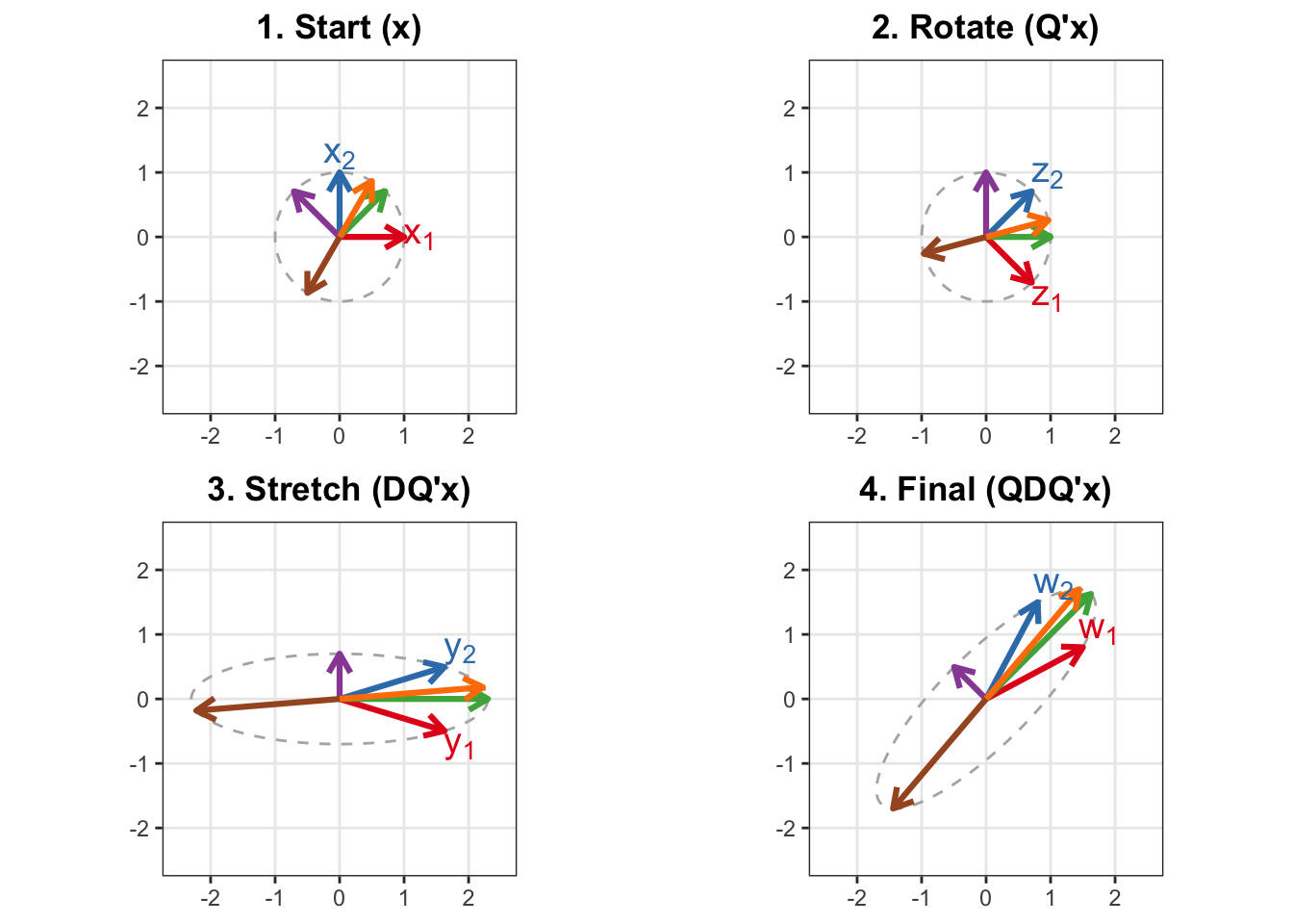
# --- 1. MATRIX SETUP ---
# Symmetric Matrix where eigenvectors are tilted
A <- matrix(c(1.5, 0.8, 0.8, 1.5), nrow = 2)

# Decomposition A = QDQ'
eig <- eigen(A)
Q <- eig$vectors
D_mat <- diag(eig$values)

# --- 2. DEFINE THE 6 VECTORS ---

# 1 & 2: Standard Axes (We will label these x1, x2)
v1 <- c(1, 0)
v2 <- c(0, 1)
# 3 & 4: Eigenvectors
v3 <- Q[,1]
v4 <- Q[,2]
# 5 & 6: Filler vectors at random angles
v5 <- c(cos(pi/3), sin(pi/3))
v6 <- c(cos(4*pi/3), sin(4*pi/3))

# Combine into starting matrix V_start
V_start <- cbind(v1, v2, v3, v4, v5, v6)

# Define 6 Distinct Colors
my_colors <- c("#E41A1C", "#377EB8", "#4DAF4A", "#984EA3", "#FF7F00", "#A65628")
names(my_colors) <- 1:6

# Background Circle Points used for reference path in all plots
theta_c <- seq(0, 2*pi, length.out = 150)
C_start <- rbind(cos(theta_c), sin(theta_c))

# --- 3. DATA PROCESSING HELPER FUNCTION ---

# This function prepares the data frames for ggplot for a given stage
prepare_data <- function(V_mat, C_mat, stage_title, label_text_pair) {
  # Prepare Vectors data frame
  df_v <- data.frame(t(V_mat))
  colnames(df_v) <- c("x", "y")
  df_v$vec_id <- factor(1:6) # Unique ID for coloring
  
  # Add labels only for vector 1 and 2
  df_v$label <- ""
  df_v$label[1] <- label_text_pair[1]
  df_v$label[2] <- label_text_pair[2]
  
  # Calculate nudge for labels based on vector direction so they don't overlap arrow tip
  df_v$nudge_x <- sign(df_v$x) * 0.25
  df_v$nudge_y <- sign(df_v$y) * 0.25
  # Don't nudge unlabelled vectors
  df_v$nudge_x[3:6] <- 0
  df_v$nudge_y[3:6] <- 0

  # Prepare Background Path data frame
  df_c <- data.frame(t(C_mat))
  colnames(df_c) <- c("px", "py")
  
  list(vecs = df_v, path = df_c, title = stage_title)
}


# --- 4. PERFORM TRANSFORMATIONS ---

# Stage 1: Start (x)
d1 <- prepare_data(V_start, C_start, 
                   "1. Start (x)", c("x[1]", "x[2]"))

# Stage 2: Rotate (Q'x)
V2 <- t(Q) %*% V_start
C2 <- t(Q) %*% C_start
d2 <- prepare_data(V2, C2, 
                   "2. Rotate (Q'x)", c("z[1]", "z[2]"))

# Stage 3: Stretch (DQ'x)
V3 <- D_mat %*% V2
C3 <- D_mat %*% C2
d3 <- prepare_data(V3, C3, 
                   "3. Stretch (DQ'x)", c("y[1]", "y[2]"))

# Stage 4: Rotate Back (QDQ'x)
V4 <- Q %*% V3
C4 <- Q %*% C3
d4 <- prepare_data(V4, C4, 
                   "4. Final (QDQ'x)", c("w[1]", "w[2]"))


# --- 5. PLOTTING FUNCTION ---

plot_stage_final <- function(data_list) {
  ggplot() +
    # Background path (gray dashed)
    geom_path(data = data_list$path, aes(x=px, y=py), 
              color="gray70", linetype="dashed") +
    # The 6 vectors
    geom_segment(data = data_list$vecs, aes(x=0, y=0, xend=x, yend=y, color=vec_id), 
                 arrow = arrow(length = unit(0.3, "cm")), size=1.1) +
    # The labels for v1 and v2 using parsed expressions for subscripts
    geom_text(data = data_list$vecs, aes(x=x, y=y, label=label, color=vec_id),
              parse = TRUE, fontface="bold", size=5,
              nudge_x = data_list$vecs$nudge_x,
              nudge_y = data_list$vecs$nudge_y) +
    scale_color_manual(values = my_colors) +
    # Fixed coordinates to ensure realistic rotation/stretching view
    coord_fixed(xlim = c(-2.5, 2.5), ylim = c(-2.5, 2.5)) +
    theme_bw() +
    theme(legend.position = "none",
          panel.grid.minor = element_blank(),
          plot.title = element_text(face="bold", hjust=0.5),
          axis.title = element_blank()) +
    labs(title = data_list$title)
}

# Generate the 4 plots
p1 <- plot_stage_final(d1)
p2 <- plot_stage_final(d2)
p3 <- plot_stage_final(d3)
p4 <- plot_stage_final(d4)

# Arrange them in a grid
grid.arrange(p1, p2, p3, p4, nrow = 2)

3.2.2 Quadratic Form

Definition 3.2 A quadratic form in \(n\) variables \(x_1, x_2, \dots, x_n\) is a scalar function defined by a symmetric matrix \(A\): \[ Q(x) = x'Ax = \sum_{i=1}^n \sum_{j=1}^n a_{ij} x_i x_j \]

3.2.3 Positive and Non-Negative Definite Matrices

Definition 3.3 (Positive and Non-Negative Definite Matrices) A symmetric matrix \(A\) is positive definite (p.d.) if: \[ x'Ax > 0 \quad \forall x \ne 0 \] It is non-negative definite (n.n.d.) if: \[ x'Ax \ge 0 \quad \forall x \]

Theorem 3.2 (Properties of Definite Matrices) Let \(A\) be a symmetric \(n \times n\) matrix with eigenvalues \(\lambda_1, \dots, \lambda_n\).

Eigenvalue Characterization:
- \(A\) is p.d. \(\iff\) all \(\lambda_i > 0\).
- \(A\) is n.n.d. \(\iff\) all \(\lambda_i \ge 0\).
Determinant and Inverse:
- If \(A\) is p.d., then \(|A| > 0\) and \(A^{-1}\) exists.
- If \(A\) is n.n.d. and singular, then \(|A| = 0\) (at least one \(\lambda_i = 0\)).
Gram Matrices (\(B'B\)): Let \(B\) be an \(n \times p\) matrix.
- If \(\text{rank}(B) = p\), then \(B'B\) is p.d.
- If \(\text{rank}(B) < p\), then \(B'B\) is n.n.d.

3.2.4 Properties of Symmetric Matrices

Theorem 3.3 (Properties of Symmetric Matrices) Let \(A\) be a symmetric matrix with spectral decomposition \(A = Q \Lambda Q'\). The following properties hold:

Trace: \(\text{tr}(A) = \sum \lambda_i\).
Determinant: \(|A| = \prod \lambda_i\).
Singularity: \(A\) is singular if and only if at least one \(\lambda_i = 0\).
Inverse: If \(A\) is non-singular (\(\lambda_i \ne 0\)), then \(A^{-1} = Q \Lambda^{-1} Q'\).
Powers: \(A^k = Q \Lambda^k Q'\).
- Square Root: \(A^{1/2} = Q \Lambda^{1/2} Q'\) (if \(\lambda_i \ge 0\)).
Spectral Representation of Quadratic Forms: The quadratic form \(x'Ax\) can be diagonalized using the eigenvectors of \(A\): \[ x'Ax = x' Q \Lambda Q' x = y' \Lambda y = \sum_{i=1}^n \lambda_i y_i^2 \] where \(y = Q'x\) represents a rotation of the coordinate system.

3.2.5 Spectral Representation of Projection Matrices

We revisit projection matrices in the context of eigenvalues.

Theorem 3.4 (Eigenvalues of Projection Matrices) A symmetric matrix \(P\) is a projection matrix (idempotent, \(P^2=P\)) if and only if its eigenvalues are either 0 or 1.

\[ P^2 x = \lambda^2 x \quad \text{and} \quad Px = \lambda x \implies \lambda^2 = \lambda \implies \lambda \in \{0, 1\} \]

For a projection matrix \(P\):

If \(x \in \text{Col}(P)\), \(Px = x\) (Eigenvalue 1).
If \(x \perp \text{Col}(P)\), \(Px = 0\) (Eigenvalue 0).
\(\text{rank}(P) = \text{tr}(P) = \sum \lambda_i\) (Count of 1s).

Example 3.1 For \(P = \frac{1}{n} J_n J_n'\), the rank is \(\text{tr}(P) = 1\).

3.3 Singular Value Decomposition (SVD)

Theorem 3.5 (Singular Value Decomposition (SVD)) Let \(X\) be an \(n \times p\) matrix with rank \(r \le \min(n, p)\). \(X\) can be decomposed into the product of three matrices:

\[ X = U \mathbf{D} V' \]

Partitioned Matrix Form

\[ X = \underset{n \times n}{(U_1, U_2)} \begin{pmatrix} \Lambda_r & O_{r \times (p-r)} \\ O_{(n-r) \times r} & O_{(n-r) \times (p-r)} \end{pmatrix} \underset{p \times p}{ \begin{pmatrix} V_1' \\ V_2' \end{pmatrix} } \]

Detailed Matrix Form

Expanding the diagonal matrix explicitly:

\[ X = \underset{n \times n}{(u_1, \dots, u_n)} \left( \begin{array}{cccc|c} \lambda_1 & 0 & \dots & 0 & \\ 0 & \lambda_2 & \dots & 0 & O_{12} \\ \vdots & \vdots & \ddots & \vdots & \\ 0 & 0 & \dots & \lambda_r & \\ \hline & O_{21} & & & O_{22} \end{array} \right) \underset{p \times p}{ \begin{pmatrix} v_1' \\ \vdots \\ v_p' \end{pmatrix} } \]

Reduced Form

\[ X = U_1 \Lambda_r V_1' = \sum_{i=1}^r \lambda_i u_i v_i' \]

Properties:

Singular Values (\(\Lambda_r\)): \(\Lambda_r = \text{diag}(\lambda_1, \dots, \lambda_r)\) contains the singular values (\(\lambda_i > 0\)), which are the square roots of the non-zero eigenvalues of \(X'X\).
Orthogonality:
- \(U\) is \(n \times n\) orthogonal (\(U'U = I_n\)).
- \(V\) is \(p \times p\) orthogonal (\(V'V = I_p\)).

3.3.0.1 Connection to Gram Matrices

The matrices \(U\) and \(V\) provide the basis vectors (eigenvectors) for the Gram matrices of \(X\).

Right Singular Vectors (\(V\)): The columns of \(V\) are the eigenvectors of the Gram matrix \(X'X\). \[ X'X = (U \Lambda V')' (U \Lambda V') = V \Lambda U' U \Lambda V' = V \Lambda^2 V' \]
- The eigenvalues of \(X'X\) are the squared singular values \(\lambda_i^2\).
Left Singular Vectors (\(U\)): The columns of \(U\) are the eigenvectors of the Gram matrix \(XX'\). \[ XX' = (U \Lambda V') (U \Lambda V')' = U \Lambda V' V \Lambda U' = U \Lambda^2 U' \]
- The eigenvalues of \(XX'\) are also \(\lambda_i^2\) (for non-zero values).

Example 3.2 (Example of SVD) Consider the matrix \(X = \begin{pmatrix} 1 & 1 \\ 2 & 2 \end{pmatrix}\).

Compute \(X'X\) and find \(V\): \[ X'X = \begin{pmatrix} 1 & 2 \\ 1 & 2 \end{pmatrix} \begin{pmatrix} 1 & 1 \\ 2 & 2 \end{pmatrix} = \begin{pmatrix} 5 & 5 \\ 5 & 5 \end{pmatrix} \]
- Eigenvalues of \(X'X\): Trace is 10, Determinant is 0. Thus, \(\mu_1 = 10, \mu_2 = 0\).
- Singular Values: \(\lambda_1 = \sqrt{10}, \lambda_2 = 0\).
- Eigenvector for \(\mu_1=10\): Normalized \(v_1 = \frac{1}{\sqrt{2}}\begin{pmatrix} 1 \\ 1 \end{pmatrix}\).
- Eigenvector for \(\mu_2=0\): Normalized \(v_2 = \frac{1}{\sqrt{2}}\begin{pmatrix} 1 \\ -1 \end{pmatrix}\).
- Therefore, \(V = \frac{1}{\sqrt{2}}\begin{pmatrix} 1 & 1 \\ 1 & -1 \end{pmatrix}\).
Compute \(XX'\) and find \(U\): \[ XX' = \begin{pmatrix} 1 & 1 \\ 2 & 2 \end{pmatrix} \begin{pmatrix} 1 & 2 \\ 1 & 2 \end{pmatrix} = \begin{pmatrix} 2 & 4 \\ 4 & 8 \end{pmatrix} \]
- Eigenvalues are again 10 and 0.
- Eigenvector for \(\mu_1=10\): Normalized \(u_1 = \frac{1}{\sqrt{5}}\begin{pmatrix} 1 \\ 2 \end{pmatrix}\).
- Eigenvector for \(\mu_2=0\): Normalized \(u_2 = \frac{1}{\sqrt{5}}\begin{pmatrix} 2 \\ -1 \end{pmatrix}\).
- Therefore, \(U = \frac{1}{\sqrt{5}}\begin{pmatrix} 1 & 2 \\ 2 & -1 \end{pmatrix}\).
Verification: \[ X = \sqrt{10} u_1 v_1' = \sqrt{10} \begin{pmatrix} \frac{1}{\sqrt{5}} \\ \frac{2}{\sqrt{5}} \end{pmatrix} \begin{pmatrix} \frac{1}{\sqrt{2}} & \frac{1}{\sqrt{2}} \end{pmatrix} = \begin{pmatrix} 1 & 1 \\ 2 & 2 \end{pmatrix} \]

3.4 Cholesky Decomposition

A symmetric matrix \(A\) has a Cholesky decomposition if and only if it is non-negative definite (i.e., \(x'Ax \ge 0\) for all \(x\)).

\[ A = B'B \]

where \(B\) is an upper triangular matrix with non-negative diagonal entries.

3.4.1 Matrix Representation of the Algorithm

To derive the algorithm, we equate the elements of \(A\) with the product of the lower triangular matrix \(B'\) and the upper triangular matrix \(B\).

For a \(3 \times 3\) matrix, this looks like:

\[ \underbrace{\begin{pmatrix} a_{11} & a_{12} & a_{13} \\ a_{21} & a_{22} & a_{23} \\ a_{31} & a_{32} & a_{33} \end{pmatrix}}_{A} = \underbrace{\begin{pmatrix} b_{11} & 0 & 0 \\ b_{12} & b_{22} & 0 \\ b_{13} & b_{23} & b_{33} \end{pmatrix}}_{B'} \underbrace{\begin{pmatrix} b_{11} & b_{12} & b_{13} \\ 0 & b_{22} & b_{23} \\ 0 & 0 & b_{33} \end{pmatrix}}_{B} \]

Multiplying the matrices on the right yields the system of equations:

\[ A = \begin{pmatrix} \mathbf{b_{11}^2} & b_{11}b_{12} & b_{11}b_{13} \\ b_{12}b_{11} & \mathbf{b_{12}^2 + b_{22}^2} & b_{12}b_{13} + b_{22}b_{23} \\ b_{13}b_{11} & b_{13}b_{12} + b_{23}b_{22} & \mathbf{b_{13}^2 + b_{23}^2 + b_{33}^2} \end{pmatrix} \]

By solving for the bolded diagonal terms and substituting known values from previous rows, we get the recursive algorithm.

Algorithm

Row 1: Solve for \(b_{11}\) using \(a_{11}\), then solve the rest of the row (\(b_{1j}\)) by division.
- \(b_{11} = \sqrt{a_{11}}\)
- \(b_{1j} = a_{1j}/b_{11}\)
Row 2: Solve for \(b_{22}\) using \(a_{22}\) and the known \(b_{12}\), then solve \(b_{2j}\).
- \(b_{22} = \sqrt{a_{22} - b_{12}^2}\)
- \(b_{2j} = (a_{2j} - b_{12}b_{1j}) / b_{22}\)
Row 3: Solve for \(b_{33}\) using \(a_{33}\) and the known \(b_{13}, b_{23}\).
- \(b_{33} = \sqrt{a_{33} - b_{13}^2 - b_{23}^2}\)

Remark. Handling the Singular Case

If \(A\) is positive semi-definite (singular), a diagonal element \(b_{ii}\) may evaluate to 0 (or a very small number close to 0 due to floating-point error). Standard algorithms often crash here because calculating off-diagonal terms involves division by \(b_{ii}\).

To handle this robustly without pivoting:

If \(b_{ii} \approx 0\), it implies that the entire remaining row \(b_{i, i:n}\) must be 0 for the matrix to remain consistent with being positive semi-definite.
The algorithm should explicitly set \(b_{ij} = 0\) for all \(j \ge i\) and proceed to the next row, rather than attempting division.

Example 3.3 (Example of Cholesky Decomposition) Consider the positive definite matrix \(A\): \[ A = \begin{pmatrix} 4 & 2 & -2 \\ 2 & 10 & 2 \\ -2 & 2 & 6 \end{pmatrix} \]

We find \(B\) such that \(A = B'B\):

First Row of B (\(b_{11}, b_{12}, b_{13}\)):
- \(b_{11} = \sqrt{4} = 2\)
- \(b_{12} = 2 / 2 = 1\)
- \(b_{13} = -2 / 2 = -1\)
Second Row of B (\(b_{22}, b_{23}\)):
- \(b_{22} = \sqrt{10 - (1)^2} = \sqrt{9} = 3\)
- \(b_{23} = (2 - (1)(-1)) / 3 = 3/3 = 1\)
Third Row of B (\(b_{33}\)):
- \(b_{33} = \sqrt{6 - (-1)^2 - (1)^2} = \sqrt{4} = 2\)

Result: \[ B = \begin{pmatrix} 2 & 1 & -1 \\ 0 & 3 & 1 \\ 0 & 0 & 2 \end{pmatrix} \]

3.4.2 Applications in Statistics

Cholesky decomposition is preferred over other methods (like LU or SVD) for symmetric positive-definite matrices because it is numerically stable and roughly twice as fast.

Solving Linear Equations

In linear regression, we solve the normal equations \((X'X)\beta = X'y\). Since \(X'X\) is symmetric and positive definite, we can decompose it as \(B'B\). The system becomes: \[ B'B\beta = X'y \] This allows us to solve for \(\beta\) using two efficient triangular substitutions (first solving \(B'z = X'y\) for \(z\), then \(B\beta = z\) for \(\beta\)) without explicitly inverting the matrix, which is computationally expensive and unstable.
Computing the Determinant

The determinant of a triangular matrix is simply the product of its diagonal entries. Therefore, the determinant of \(A\) can be computed instantly from \(B\): \[ \det(A) = \det(B'B) = \det(B')\det(B) = \left(\prod_{i=1}^n b_{ii}\right)^2 \] This is widely used in Maximum Likelihood Estimation (e.g., REML in mixed models) where log-determinants of large covariance matrices are required.
Generating Multivariate Normal Random Variables

To generate a random vector \(Y \sim N(\mu, \Sigma)\), we first generate a vector of independent standard normal variables \(Z \sim N(0, I)\). Using the Cholesky decomposition \(\Sigma = B'B\): \[ Y = \mu + B'Z \] The covariance of \(Y\) is confirmed by \(\text{Cov}(Y) = B' \text{Cov}(Z) B = B' I B = B'B = \Sigma\). This is the standard method used by functions like mvrnorm in R.