6  Likelihood-based Tests

6.1 The Geometry of Mahalanobis Distance

6.1.1 Pythagorean Theorem for Mahalanobis Distance

Definitions and Setup

Let \(x\) be a random vector partitioned as \(x = (x_0, x_1)^T\), and let \(\mu\) be its corresponding center vector \(\mu = (\mu_0, \mu_1)^T\). Let \(\Sigma\) be a symmetric, positive-definite covariance matrix governing the joint space, partitioned into corresponding blocks:

\[ \Sigma = \begin{pmatrix} \Sigma_{00} & \Sigma_{01} \\ \Sigma_{10} & \Sigma_{11} \end{pmatrix} \]

Define the generalized squared Mahalanobis distance of any vector \(v\) to a center \(c\) with respect to a positive-definite matrix \(S\) as:

\[ D^2(v, c, S) = (v - c)^T S^{-1} (v - c) \]

For a symmetric, positive-definite matrix \(S\), the Mahalanobis inner product between two vectors \(u\) and \(v\) is defined as \(\langle u, v \rangle_{S^{-1}} = u^T S^{-1} v\). Two vectors are orthogonal in this space if their inner product is zero.

Define the conditional expectation (the linear regression surface) of \(x_1\) given \(x_0\) as \(\mu_{1|0}(x_0)\):

\[ \mu_{1|0}(x_0) = \mu_1 + \Sigma_{10}\Sigma_{00}^{-1}(x_0 - \mu_0) \]

Define the conditional covariance matrix (the Schur complement of \(\Sigma_{00}\) in \(\Sigma\)) as \(\Sigma_{1|0}\):

\[ \Sigma_{1|0} = \Sigma_{11} - \Sigma_{10}\Sigma_{00}^{-1}\Sigma_{01} \]

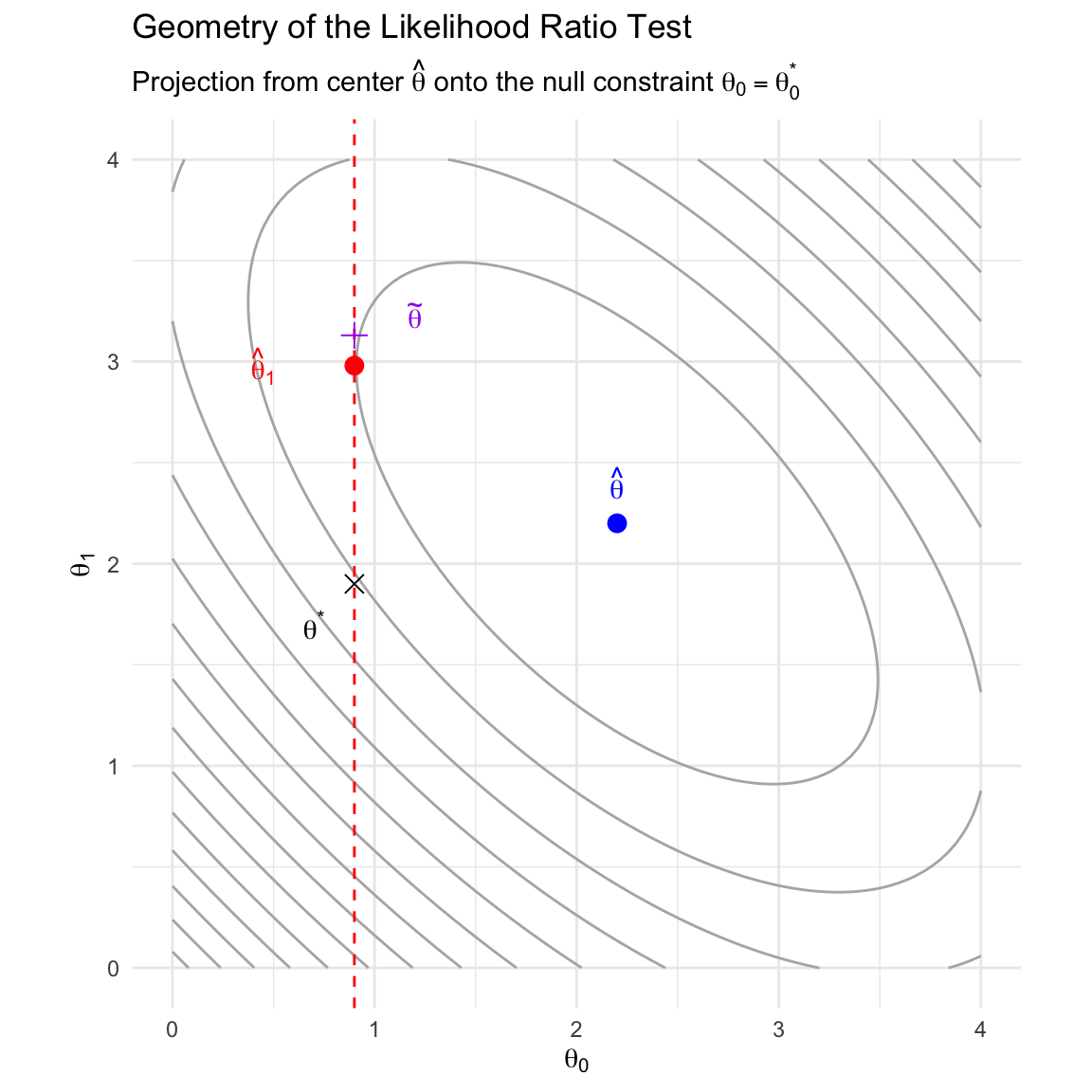
Finally, define the Projection Point (\(\tilde{x}\)) as the point where \(x\) projects exactly onto the regression surface: \(\tilde{x} = (x_0, \tilde{x}_1)^T\), where \(\tilde{x}_1 = \mu_{1|0}(x_0)\).


Lemma 6.1 (Fundamental Orthogonal Decomposition Lemma) Any deviation from the center, \((x - \mu)\), can be expressed as the sum of a conditional residual vector \((x - \tilde{x})\) and a marginal projection vector \((\tilde{x} - \mu)\).

These two vectors are strictly orthogonal with respect to the precision matrix \(\Sigma^{-1}\): \[ (x - \tilde{x})^T \Sigma^{-1} (\tilde{x} - \mu) = 0 \]

Furthermore, the joint Mahalanobis distances of these individual vectors perfectly isolate the conditional and marginal spaces:

  1. \((x - \tilde{x})^T \Sigma^{-1} (x - \tilde{x}) = D^2(x_1, \tilde{x}_1, \Sigma_{1|0})\)
  2. \((\tilde{x} - \mu)^T \Sigma^{-1} (\tilde{x} - \mu) = D^2(x_0, \mu_0, \Sigma_{00})\)

Proof. Proof via Block Factorization

We can express the partitioned covariance matrix \(\Sigma\) using a block \(LDL^T\) factorization. The precision matrix is then \(\Sigma^{-1} = (L^{-1})^T D^{-1} L^{-1}\), where:

\[ L^{-1} = \begin{pmatrix} I & 0 \\ -\Sigma_{10}\Sigma_{00}^{-1} & I \end{pmatrix}, \quad D^{-1} = \begin{pmatrix} \Sigma_{00}^{-1} & 0 \\ 0 & \Sigma_{1|0}^{-1} \end{pmatrix} \]

Evaluating Mahalanobis inner products with \(\Sigma^{-1}\) is equivalent to applying the shearing transformation \(L^{-1}\) to the vectors, and then taking their inner product with respect to the block-diagonal metric \(D^{-1}\). Let us evaluate the transformed vectors for the residual \(u = (x - \tilde{x})\) and the projection \(v = (\tilde{x} - \mu)\).

  1. Transforming the Residual Vector (\(L^{-1}u\)):

\[ L^{-1} (x - \tilde{x}) = \begin{pmatrix} I & 0 \\ -\Sigma_{10}\Sigma_{00}^{-1} & I \end{pmatrix} \begin{pmatrix} 0 \\ x_1 - \tilde{x}_1 \end{pmatrix} = \begin{pmatrix} 0 \\ x_1 - \tilde{x}_1 \end{pmatrix} \] The transformation leaves the residual vector unchanged; it lies entirely in the conditional subspace.

  1. Transforming the Projection Vector (\(L^{-1}v\)):

\[ L^{-1} (\tilde{x} - \mu) = \begin{pmatrix} I & 0 \\ -\Sigma_{10}\Sigma_{00}^{-1} & I \end{pmatrix} \begin{pmatrix} x_0 - \mu_0 \\ \Sigma_{10}\Sigma_{00}^{-1}(x_0 - \mu_0) \end{pmatrix} = \begin{pmatrix} x_0 - \mu_0 \\ 0 \end{pmatrix} \] The transformation cleanly removes the induced correlation, flattening the projection vector so it lies entirely in the marginal subspace.

Evaluating the Inner Products: Because \(D^{-1}\) is block-diagonal, the inner product of these transformed vectors is simply the sum of the inner products of their corresponding blocks:

\[ (x - \tilde{x})^T \Sigma^{-1} (\tilde{x} - \mu) = \begin{pmatrix} 0 \\ x_1 - \tilde{x}_1 \end{pmatrix}^T \begin{pmatrix} \Sigma_{00}^{-1} & 0 \\ 0 & \Sigma_{1|0}^{-1} \end{pmatrix} \begin{pmatrix} x_0 - \mu_0 \\ 0 \end{pmatrix} = 0 + 0 = 0 \] This proves strict orthogonality.

Applying the same logic to the self-inner products evaluates the quadratic forms: \[ (x - \tilde{x})^T \Sigma^{-1} (x - \tilde{x}) = \begin{pmatrix} 0 \\ x_1 - \tilde{x}_1 \end{pmatrix}^T \begin{pmatrix} \Sigma_{00}^{-1} & 0 \\ 0 & \Sigma_{1|0}^{-1} \end{pmatrix} \begin{pmatrix} 0 \\ x_1 - \tilde{x}_1 \end{pmatrix} = (x_1 - \tilde{x}_1)^T \Sigma_{1|0}^{-1} (x_1 - \tilde{x}_1) \] \[ (\tilde{x} - \mu)^T \Sigma^{-1} (\tilde{x} - \mu) = \begin{pmatrix} x_0 - \mu_0 \\ 0 \end{pmatrix}^T \begin{pmatrix} \Sigma_{00}^{-1} & 0 \\ 0 & \Sigma_{1|0}^{-1} \end{pmatrix} \begin{pmatrix} x_0 - \mu_0 \\ 0 \end{pmatrix} = (x_0 - \mu_0)^T \Sigma_{00}^{-1} (x_0 - \mu_0) \] which yields exactly \(D^2(x_1, \tilde{x}_1, \Sigma_{1|0})\) and \(D^2(x_0, \mu_0, \Sigma_{00})\), respectively.


Theorem 6.1 (The Generalized Pythagorean Decomposition for Mahalanobis Distance) For any point \(x\), the total joint squared Mahalanobis distance from \(x\) to the center \(\mu\) decomposes precisely into the sum of the squared distances between \(x\) and its projection \(\tilde{x}\) (the Conditional Residual), and between \(\tilde{x}\) and the center \(\mu\) (the Marginal Projection):

\[ D^2(x, \mu, \Sigma) = D^2(x, \tilde{x}, \Sigma) + D^2(\tilde{x}, \mu, \Sigma) \]

which, mapping to the marginal and conditional subspaces, is equivalent to:

\[ D^2(x, \mu, \Sigma) = D^2(x_1, \tilde{x}_1, \Sigma_{1|0}) + D^2(x_0, \mu_0, \Sigma_{00}) \]

Proof. Proof

We construct the vector from the origin to the target as the sum of the residual and the projection: \[ x - \mu = (x - \tilde{x}) + (\tilde{x} - \mu) \]

We evaluate the total joint distance by expanding the quadratic form: \[ D^2(x, \mu, \Sigma) = \Big( (x - \tilde{x}) + (\tilde{x} - \mu) \Big)^T \Sigma^{-1} \Big( (x - \tilde{x}) + (\tilde{x} - \mu) \Big) \]

\[ = (x - \tilde{x})^T \Sigma^{-1} (x - \tilde{x}) + (\tilde{x} - \mu)^T \Sigma^{-1} (\tilde{x} - \mu) + 2 (x - \tilde{x})^T \Sigma^{-1} (\tilde{x} - \mu) \]

By the Fundamental Orthogonal Decomposition Lemma, the cross-term evaluates to zero due to orthogonality, leaving only the isolated quadratic forms:

\[ D^2(x, \mu, \Sigma) = (x - \tilde{x})^T \Sigma^{-1} (x - \tilde{x}) + (\tilde{x} - \mu)^T \Sigma^{-1} (\tilde{x} - \mu) \]

This is exactly \(D^2(x, \tilde{x}, \Sigma) + D^2(\tilde{x}, \mu, \Sigma)\). Furthermore, as established by the Lemma, substituting the subspace identities for these two terms yields \(D^2(x_1, \tilde{x}_1, \Sigma_{1|0}) + D^2(x_0, \mu_0, \Sigma_{00})\).

6.1.2 Interactive Illustration

#| '!! shinylive warning !!': |
#|   shinylive does not work in self-contained HTML documents.
#|   Please set `embed-resources: false` in your metadata.
#| standalone: true
#| viewerHeight: 750
#| echo: false
#| column: screen
#| label: fig-MD-decomp-unified

library(shiny)
library(ggplot2)

ui <- fluidPage(
  titlePanel("Pythagorean Decomposition of Mahalanobis Distance"),
  
  # A relative container holding the plot and absolute panels
  div(style = "position: relative;",
      
      plotOutput("distPlot", height = "700px", width = "100%"),
      
      # Floating Control Panel (Top Left)
      absolutePanel(
        top = 10, left = 10, width = 320, draggable = TRUE,
        style = "background-color: rgba(255, 255, 255, 0.85); padding: 10px 15px; border-radius: 8px; border: 1px solid #ccc; box-shadow: 2px 2px 10px rgba(0,0,0,0.1);",
        
        h4("Parameters", style = "margin-top: 0; margin-bottom: 10px; font-size: 16px;"),
        
        fluidRow(
          column(6, sliderInput("mu_0", "\\(\\mu_0\\)", min = 0, max = 5, value = 2.2, step = 0.1, ticks = FALSE)),
          column(6, sliderInput("mu_1", "\\(\\mu_1\\)", min = 0, max = 5, value = 2.2, step = 0.1, ticks = FALSE))
        ),
        fluidRow(
          column(6, sliderInput("x_0", "\\(x_0\\)", min = 0, max = 5, value = 0.9, step = 0.1, ticks = FALSE)),
          column(6, sliderInput("x_1", "\\(x_1\\)", min = 0, max = 5, value = 1.9, step = 0.1, ticks = FALSE))
        ),
        hr(style = "margin: 5px 0; border-top: 1px solid #ddd;"),
        fluidRow(
          column(6, sliderInput("sigma_0", "\\(\\sigma_0\\)", min = 0.5, max = 3, value = 1.25, step = 0.05, ticks = FALSE)),
          column(6, sliderInput("sigma_1", "\\(\\sigma_1\\)", min = 0.5, max = 3, value = 1.25, step = 0.05, ticks = FALSE))
        ),
        sliderInput("rho", "Correlation \\(\\rho\\)", min = -0.95, max = 0.95, value = -0.6, step = 0.05, ticks = FALSE)
      ),
      
      # Floating Legend Panel (Bottom Right)
      absolutePanel(
        bottom = 20, right = 20, width = 340, draggable = TRUE,
        style = "background-color: rgba(255, 255, 255, 0.9); padding: 10px; border-radius: 8px; border: 1px solid #ccc; box-shadow: 2px 2px 10px rgba(0,0,0,0.1);",
        uiOutput("legendUI")
      )
  )
)

server <- function(input, output, session) {
  
  # Reactive calculations
  calc_data <- reactive({
    mu <- c(input$mu_0, input$mu_1)
    x <- c(input$x_0, input$x_1)
    
    # Construct Covariance Matrix
    Sigma <- matrix(c(
      input$sigma_0^2, 
      input$rho * input$sigma_0 * input$sigma_1, 
      input$rho * input$sigma_0 * input$sigma_1, 
      input$sigma_1^2
    ), nrow = 2)
    
    Sigma_inv <- solve(Sigma)
    
    # Marginal and Conditional variances
    Sigma_00 <- Sigma[1, 1]
    Sigma_1given0 <- Sigma[2, 2] - (Sigma[1, 2]^2) / Sigma[1, 1]
    
    # Conditional Mean
    mu_1given0 <- mu[2] + (Sigma[1, 2] / Sigma[1, 1]) * (x[1] - mu[1])
    
    # Projected Point p = \tilde{x} = (x_0, \mu_{1|0}(x_0))
    x_tilde <- c(x[1], mu_1given0)
    
    # Calculate Distances
    diff_total <- x - mu
    d2_total <- as.numeric(t(diff_total) %*% Sigma_inv %*% diff_total)
    
    # By theorem, marginal maps to D^2(\tilde{x}, \mu, \Sigma)
    d2_marg <- (x[1] - mu[1])^2 / Sigma_00 
    
    # By theorem, conditional maps to D^2(x, \tilde{x}, \Sigma)
    d2_cond <- (x[2] - mu_1given0)^2 / Sigma_1given0
    
    list(mu = mu, x = x, x_tilde = x_tilde, Sigma = Sigma, Sigma_inv = Sigma_inv, 
         d2_total = d2_total, d2_marg = d2_marg, d2_cond = d2_cond)
  })
  
  output$legendUI <- renderUI({
    res <- calc_data()
    withMathJax(
      HTML(paste0(
        "<div style='font-size: 14px;'>",
        "<b>Distance Legend</b><br><br>",
        "<span style='color: black;'><b>Total:</b> \\( D^2(x, \\mu, \\Sigma) = \\) ", round(res$d2_total, 2), "</span><br>",
        "<span style='color: blue;'><b>Marginal:</b> \\( D^2(\\tilde{x}, \\mu, \\Sigma) = \\) ", round(res$d2_marg, 2), "</span><br>",
        "<span style='color: red;'><b>Conditional:</b> \\( D^2(x, \\tilde{x}, \\Sigma) = \\) ", round(res$d2_cond, 2), "</span>",
        "</div>"
      ))
    )
  })
  
  output$distPlot <- renderPlot({
    res <- calc_data()
    mu <- res$mu; x <- res$x; x_tilde <- res$x_tilde; Sigma <- res$Sigma; Sigma_inv <- res$Sigma_inv
    
    # Generate grid for quadratic contours (extended for fixed bounds)
    grid_vals <- seq(-2, 7, length.out = 100)
    grid <- expand.grid(x0 = grid_vals, x1 = grid_vals)
    grid$z <- apply(grid, 1, function(row) {
      diff <- row - mu
      as.numeric(t(diff) %*% Sigma_inv %*% diff)
    })
    
    # Regression surface line parameters
    slope <- Sigma[1, 2] / Sigma[1, 1]
    intercept <- mu[2] - slope * mu[1]
    
    # Midpoints for labels
    mid_marg <- (mu + x_tilde) / 2
    mid_cond <- (x_tilde + x) / 2
    mid_total <- (mu + x) / 2
    
    ggplot(grid, aes(x = x0, y = x1)) +
      # Contours
      geom_contour(aes(z = z), bins = 25, color = "gray85") +
      
      # The Regression Surface (Light Blue Line extending across plot)
      geom_abline(intercept = intercept, slope = slope, color = "lightblue", linewidth = 2, alpha = 0.5) +
      
      # The Distance Segments
      geom_segment(aes(x = mu[1], y = mu[2], xend = x_tilde[1], yend = x_tilde[2]), color = "blue", linewidth = 1.2) +
      geom_segment(aes(x = x_tilde[1], y = x_tilde[2], xend = x[1], yend = x[2]), color = "red", linewidth = 1.2) +
      geom_segment(aes(x = mu[1], y = mu[2], xend = x[1], yend = x[2]), color = "black", linetype = "dashed", linewidth = 1) +
      
      # Labels on Segments using unified notation
      annotate("text", x = mid_marg[1] + 0.25, y = mid_marg[2] - 0.25, label = "D^2*(list(tilde(x), mu, Sigma))", parse = TRUE, color = "blue", size = 5) +
      annotate("text", x = mid_cond[1] + 0.35, y = mid_cond[2], label = "D^2*(list(x, tilde(x), Sigma))", parse = TRUE, color = "red", size = 5) +
      annotate("text", x = mid_total[1] - 0.25, y = mid_total[2] + 0.25, label = "D^2*(list(x, mu, Sigma))", parse = TRUE, color = "black", size = 5) +
      
      # Points and their labels
      annotate("point", x = mu[1], y = mu[2], color = "blue", size = 4) +
      annotate("text", x = mu[1] - 0.2, y = mu[2] + 0.2, label = "mu", parse = TRUE, color = "blue", size = 6) +
      
      annotate("point", x = x_tilde[1], y = x_tilde[2], color = "purple", shape = 3, size = 4, stroke = 2) +
      annotate("text", x = x_tilde[1] + 0.3, y = x_tilde[2] - 0.2, label = "tilde(x)", parse = TRUE, color = "purple", size = 6) +
      
      annotate("point", x = x[1], y = x[2], color = "black", shape = 4, size = 4, stroke = 2) +
      annotate("text", x = x[1] - 0.15, y = x[2] + 0.2, label = "x", parse = TRUE, size = 6) +
      
      # Strict Fixed Coordinates to prevent re-shaping
      coord_fixed(xlim = c(-1, 6), ylim = c(-1, 6), expand = FALSE) +
      labs(x = expression(x[0]), y = expression(x[1])) +
      theme_minimal(base_size = 16) +
      theme(panel.grid.minor = element_blank())
  })
}

shinyApp(ui, server)

6.2 Likelihood Ratio Test for General Nested Models

Theorem 6.2 (Wilks’ Theorem for General Nested Models) Let \(\mathbf{Y} = (Y_1, \dots, Y_n)\) be an i.i.d. sample from a distribution \(f(\mathbf{y}; \boldsymbol{\theta})\) with \(\boldsymbol{\theta} \in \Theta \subseteq \mathbb{R}^p\). Let \(\Theta_0\) be a lower-dimensional subspace of \(\Theta\) defined by \(q\) independent constraints, such that \(\dim(\Theta_0) = p - q\).

Consider testing the nested hypotheses:

\[ H_0: \boldsymbol{\theta}_0 = \boldsymbol{\theta}_0^* \quad \text{vs} \quad H_1: \boldsymbol{\theta}_0 \neq \boldsymbol{\theta}_0^* \]

Let \(\boldsymbol{\theta}^* = (\boldsymbol{\theta}_0^*, \boldsymbol{\theta}_1^*)^T\) be the true parameter vector generating the data under \(H_0\). Let \(\hat{\boldsymbol{\theta}}\) be the unrestricted Maximum Likelihood Estimator (MLE) over \(\Theta\), and let \(\tilde{\boldsymbol{\theta}} = (\boldsymbol{\theta}_0^*, \tilde{\boldsymbol{\theta}}_1)^T\) be the restricted MLE over \(\Theta_0\).

The likelihood ratio test statistic \(D\) is defined as the difference between the unrestricted and restricted maximum log-likelihoods:

\[ D = 2 \left[ \ell(\hat{\boldsymbol{\theta}}) - \ell(\tilde{\boldsymbol{\theta}}) \right] \]

Under \(H_0\), as \(n \to \infty\), the statistic \(D\) converges in distribution to a chi-square distribution with degrees of freedom equal to the number of constraints:

\[ D \xrightarrow{d} \chi^2_q \]

Proof.

  1. Mapping Likelihood to Mahalanobis Geometry

By a second-order Taylor expansion around the unrestricted peak \(\hat{\boldsymbol{\theta}}\), log-likelihood deviances are asymptotically equivalent to squared Mahalanobis distances. The center of this space is the unrestricted MLE, and the metric is the inverse Fisher Information matrix \(\Sigma = \mathcal{I}^{-1}\).

We map the likelihood parameters directly to our geometric definitions (\(x, \mu, \tilde{x}\)):

  • The Origin (\(\mu \to \hat{\boldsymbol{\theta}}\)): The global MLE sits at the center of the quadratic contours.
  • The Target (\(x \to \boldsymbol{\theta}^*\)): The true parameter value being evaluated.
  • The Projection (\(\tilde{x} \to \tilde{\boldsymbol{\theta}}\)): The restricted MLE maximizes the likelihood given \(\boldsymbol{\theta}_0^*\). Geometrically, it minimizes the distance to the center \(\hat{\boldsymbol{\theta}}\) subject to the null constraint, which strictly defines it as the projection of \(x\) onto the regression surface: \(\tilde{\boldsymbol{\theta}}_1 = \mu_{1|0}(\boldsymbol{\theta}_0^*)\).
  1. Evaluating the Deviances

Using this mapping, we can express the total deviance (\(D_1\)), the restricted deviance (\(D_0\)), and the Wilks statistic (\(D\)) strictly as geometric distances:

  • Total Deviance: \(D_1 = 2[\ell(\hat{\boldsymbol{\theta}}) - \ell(\boldsymbol{\theta}^*)] \approx D^2(\boldsymbol{\theta}^*, \hat{\boldsymbol{\theta}}, \Sigma) \iff D^2(x, \mu, \Sigma)\)
  • Restricted Deviance: \(D_0 = 2[\ell(\tilde{\boldsymbol{\theta}}) - \ell(\boldsymbol{\theta}^*)] \approx D^2(\boldsymbol{\theta}^*, \tilde{\boldsymbol{\theta}}, \Sigma) \iff D^2(x, \tilde{x}, \Sigma)\)
  • Wilks Statistic: \(D = 2[\ell(\hat{\boldsymbol{\theta}}) - \ell(\tilde{\boldsymbol{\theta}})] \approx D^2(\tilde{\boldsymbol{\theta}}, \hat{\boldsymbol{\theta}}, \Sigma) \iff D^2(\tilde{x}, \mu, \Sigma)\)
  1. The Pythagorean Identity and Marginal Decomposition

By the Generalized Pythagorean Decomposition, we know the distances strictly relate via: \[ D^2(x, \mu, \Sigma) = D^2(x, \tilde{x}, \Sigma) + D^2(\tilde{x}, \mu, \Sigma) \] which confirms the algebraic identity of the likelihoods: \(D_1 \approx D_0 + D\).

Furthermore, Wilks’ statistic \(D\) is precisely the Marginal Projection component: \(D^2(\tilde{x}, \mu, \Sigma)\). According to the Fundamental Orthogonal Decomposition Lemma, this projection perfectly isolates the marginal distance of the constrained block:

\[ D \approx D^2(\tilde{\boldsymbol{\theta}}, \hat{\boldsymbol{\theta}}, \Sigma) = D^2(\boldsymbol{\theta}_0^*, \hat{\boldsymbol{\theta}}_0, \Sigma_{00}) = (\hat{\boldsymbol{\theta}}_0 - \boldsymbol{\theta}_0^*)^T \Sigma_{00}^{-1} (\hat{\boldsymbol{\theta}}_0 - \boldsymbol{\theta}_0^*) \]

  1. Asymptotic Distribution

Under \(H_0\), the asymptotic normality of the unrestricted MLE implies \(\sqrt{n}(\hat{\boldsymbol{\theta}}_0 - \boldsymbol{\theta}_0^*) \xrightarrow{d} N(\mathbf{0}, \Sigma_{00})\). Therefore, the isolated quadratic form \(D\) follows a chi-square distribution with \(q\) degrees of freedom:

\[ D \xrightarrow{d} \chi^2_q \]

Remark (Geometric Intuition). By centering the Mahalanobis space at the unrestricted MLE \(\hat{\boldsymbol{\theta}}\), the proof of Wilks’ Theorem collapses into a trivial geometric observation. The restricted MLE \(\tilde{\boldsymbol{\theta}}\) is simply the projection of the true parameter \(\boldsymbol{\theta}^*\) onto the regression surface. The Wilks statistic \(D\) measures the squared length of the projection leg of the resulting right triangle. Because it is a projection onto the marginal subspace, it depends only on the parameters of interest, entirely stripping away the nuisance parameters.

Diagram to Illustrate Wilks’ Theorem

The following R code visualizes the likelihood ratio test as a projection. We illustrate the unrestricted MLE \(\hat{\boldsymbol{\theta}}\) (the center of the contours), the hypothesized true value \(\boldsymbol{\theta}^*\), the geometric center \(\hat{\boldsymbol{\theta}}_{1, \Sigma}\), and a jittered point representing the actual restricted MLE \(\tilde{\boldsymbol{\theta}}_1\).

Code
library(ggplot2)

# 1. Setup parameters and Fisher Information
theta_hat <- c(2.2, 2.2)      # The Peak (Unrestricted MLE center)
theta_star <- c(0.9, 1.9)     # Hypothesized true value 
I <- matrix(c(1, 0.6, 0.6, 1), nrow = 2) # Curvature

# 2. Calculate the geometric center hat(theta)_{1, Sigma}

# Starting from the center hat(theta)_1, we adjust by the displacement in theta_0
delta_theta_0 <- theta_star[1] - theta_hat[1]
theta_hat_1_Sigma <- theta_hat[2] - (1/I[2,2]) * I[2,1] * delta_theta_0
p_projected <- c(theta_star[1], theta_hat_1_Sigma)

# 3. Create tilde(theta)_1 by adding small non-quadratic jitter to the projected center
set.seed(42)
theta_tilde <- c(theta_star[1], theta_hat_1_Sigma + 0.15) 

# 4. Generate grid for quadratic log-likelihood contours centered at theta_hat
grid_vals <- seq(0, 4, length.out = 100)
grid <- expand.grid(theta0 = grid_vals, theta1 = grid_vals)
grid$z <- apply(grid, 1, function(p) {
  diff <- p - theta_hat
  -0.5 * t(diff) %*% I %*% diff
})

# 5. Plot
ggplot(grid, aes(x = theta0, y = theta1)) +
  geom_contour(aes(z = z), bins = 15, color = "gray70") +
  geom_vline(xintercept = theta_star[1], linetype = "dashed", color = "red") +
  # Unrestricted MLE (The Center)
  annotate("point", x = theta_hat[1], y = theta_hat[2], color = "blue", size = 3) +
  annotate("text", x = theta_hat[1], y = theta_hat[2] + 0.2, 
           label = "hat(theta)", parse = TRUE, color = "blue") +
  # Projected Nuisance Center (hat(theta)[1, Sigma])
  annotate("point", x = p_projected[1], y = p_projected[2], color = "red", size = 3) +
  annotate("text", x = p_projected[1] - 0.45, y = p_projected[2], 
           label = "hat(theta)[1, Sigma]", parse = TRUE, color = "red") +
  # Restricted MLE (tilde(theta))
  annotate("point", x = theta_tilde[1], y = theta_tilde[2], color = "purple", shape = 3, size = 3) +
  annotate("text", x = theta_tilde[1] + 0.3, y = theta_tilde[2] + 0.1, 
           label = "tilde(theta)", parse = TRUE, color = "purple") +
  # Hypothesized Point (theta^*)
  annotate("point", x = theta_star[1], y = theta_star[2], color = "black", shape = 4, size = 3) +
  annotate("text", x = theta_star[1] - 0.2, y = theta_star[2] - 0.2, 
           label = "theta^'*'", parse = TRUE) +
  labs(title = "Geometry of the Likelihood Ratio Test",
       subtitle = expression(paste("Projection from center ", hat(theta), " onto the null constraint ", theta[0] == theta[0]^"*")),
       x = expression(theta[0]), y = expression(theta[1])) +
  theme_minimal() + 
  coord_fixed()
Figure 6.1: The geometry of restricted optimization. Blue dot is the unrestricted MLE (center). The red dot represents the projected nuisance parameter center on the null line. The purple cross is the restricted MLE.

Example 6.1 LRT for Normal Mean with Unknown Variance

Let \(X_1, \dots, X_n \overset{i.i.d.}{\sim} N(\mu, \sigma^2)\) where both \(\mu\) and \(\sigma^2\) are unknown. The parameter vector is \(\theta = (\mu, \sigma^2)\). We wish to test: \[ H_0: \mu = \mu_0 \quad \text{vs} \quad H_1: \mu \neq \mu_0 \]

  1. Find the Maximum Likelihood Estimators: The log-likelihood function is \(\ell(\mu, \sigma^2) = -\frac{n}{2}\ln(2\pi) - \frac{n}{2}\ln(\sigma^2) - \frac{1}{2\sigma^2}\sum_{i=1}^n (x_i - \mu)^2\).

    • Unrestricted MLEs (\(\hat{\theta}\)): \(\hat{\mu} = \overline{X}, \quad \hat{\sigma}^2 = \frac{1}{n}\sum_{i=1}^n (X_i - \overline{X})^2\). The maximized log-likelihood is: \[ \ell(\hat{\mu}, \hat{\sigma}^2) = -\frac{n}{2}\ln(2\pi) - \frac{n}{2}\ln(\hat{\sigma}^2) - \frac{n}{2} \]

    • Restricted MLEs (\(\hat{\theta}_0\)): Under \(H_0\), \(\hat{\mu}_0 = \mu_0, \quad \hat{\sigma}_0^2 = \frac{1}{n}\sum_{i=1}^n (X_i - \mu_0)^2\). The restricted maximized log-likelihood is: \[ \ell(\hat{\mu}_0, \hat{\sigma}_0^2) = -\frac{n}{2}\ln(2\pi) - \frac{n}{2}\ln(\hat{\sigma}_0^2) - \frac{n}{2} \]

  2. Define the Test Statistic \(D\): The test statistic \(D\) is defined as twice the difference between the unrestricted and restricted log-likelihoods:

\[ D = 2 \left[ \ell(\hat{\mu}, \hat{\sigma}^2) - \ell(\hat{\mu}_0, \hat{\sigma}_0^2) \right] \] Substituting the expressions above, the constant terms cancel out: \[ D = 2 \left[ -\frac{n}{2}\ln(\hat{\sigma}^2) - \left( -\frac{n}{2}\ln(\hat{\sigma}_0^2) \right) \right] = n \ln \left( \frac{\hat{\sigma}_0^2}{\hat{\sigma}^2} \right) \]

  1. Relate to the t-statistic: Using the sum of squares decomposition \(\hat{\sigma}_0^2 = \hat{\sigma}^2 + (\overline{X} - \mu_0)^2\), we have:

\[ \frac{\hat{\sigma}_0^2}{\hat{\sigma}^2} = 1 + \frac{(\overline{X} - \mu_0)^2}{\hat{\sigma}^2} \] Substituting the t-statistic \(T = \frac{\overline{X} - \mu_0}{S/\sqrt{n}}\), where \(S^2 = \frac{n}{n-1}\hat{\sigma}^2\), we find: \[ \frac{(\overline{X} - \mu_0)^2}{\hat{\sigma}^2} = \frac{T^2}{n-1} \] Thus, \(D\) is a monotone increasing function of \(T^2\): \[ D = n \ln \left( 1 + \frac{T^2}{n-1} \right) \] Rejecting \(H_0\) for large \(D\) is equivalent to rejecting for large \(|T|\).

  1. Asymptotic Distribution (Wilks’ Theorem): By Wilks’ Theorem, \(D \xrightarrow{d} \chi^2_1\). For large \(n\), using the approximation \(\ln(1+x) \approx x\):

\[ D = n \ln \left( 1 + \frac{T^2}{n-1} \right) \approx n \left( \frac{T^2}{n-1} \right) \approx T^2 \]

As \(n \to \infty\), \(T^2 \xrightarrow{d} \chi^2_1\), confirming the theorem.

6.3 Wald’s Theorem for Testing Parameter Restrictions

The Wald Test evaluates the distance between the unrestricted Maximum Likelihood Estimator (MLE) and the null hypothesis value, standardized by the curvature of the log-likelihood at the unrestricted estimate. Unlike the Score test, the Wald test requires estimating the full, unrestricted model.

Theorem 6.3 (Asymptotic Distribution of the Wald Statistic) Let \(\mathbf{Y} = (Y_1, \dots, Y_n)\) be an i.i.d. sample from a regular family of distributions with parameters \(\boldsymbol{\theta} \in \Theta \subseteq \mathbb{R}^{p}\). Partition the parameter vector as \(\boldsymbol{\theta} = (\boldsymbol{\theta}_0^T, \boldsymbol{\theta}_1^T)^T\), where \(\boldsymbol{\theta}_0\) is the \(q\)-dimensional parameter of interest and \(\boldsymbol{\theta}_1\) is the \((p-q)\)-dimensional nuisance parameter. Consider the test: \[ H_0: \boldsymbol{\theta}_0 = \boldsymbol{\theta}_0^* \quad \text{vs} \quad H_1: \boldsymbol{\theta}_0 \neq \boldsymbol{\theta}_0^* \]

Let \(\hat{\boldsymbol{\theta}} = (\hat{\boldsymbol{\theta}}_0^T, \hat{\boldsymbol{\theta}}_1^T)^T\) be the unrestricted MLE under \(H_1\). Let \(\Sigma(\boldsymbol{\theta}) = \mathcal{I}^{-1}(\boldsymbol{\theta})\) be the asymptotic covariance matrix of the unrestricted MLE, where \(\mathcal{I}(\boldsymbol{\theta})\) is the expected Fisher Information matrix, and let \(\Sigma_{00}\) denote its top-left \(q \times q\) marginal block.

The Wald statistic is defined as the quadratic form: \[ W = (\hat{\boldsymbol{\theta}}_0 - \boldsymbol{\theta}_0^*)^T \Sigma_{00}^{-1}(\hat{\boldsymbol{\theta}}) (\hat{\boldsymbol{\theta}}_0 - \boldsymbol{\theta}_0^*) \]

Under standard regularity conditions, if \(H_0\) is true, as \(n \to \infty\): \[ W \xrightarrow{d} \chi^2_q \] where \(q\) is the dimension of the parameter of interest \(\boldsymbol{\theta}_0\).

Proof. Algebraic Proof via Mahalanobis Decomposition

We can derive the Wald statistic directly by borrowing the geometric decomposition used in Wilks’ Theorem, isolating the marginal behavior of the unrestricted MLE.

  1. The Total Mahalanobis Distance

By standard large-sample theory, the unrestricted MLE \(\hat{\boldsymbol{\theta}}\) is asymptotically normal. Its asymptotic covariance matrix is \(\Sigma = \mathcal{I}^{-1}(\boldsymbol{\theta})\). The total squared Mahalanobis distance between the unrestricted MLE \(\hat{\boldsymbol{\theta}}\) and the full hypothesized parameter vector \(\boldsymbol{\theta}^* = ({\boldsymbol{\theta}_0^*}^T, {\boldsymbol{\theta}_1^*}^T)^T\) under the precision metric \(\Sigma^{-1}\) is: \[ D_{total} = (\hat{\boldsymbol{\theta}} - \boldsymbol{\theta}^*)^T \Sigma^{-1} (\hat{\boldsymbol{\theta}} - \boldsymbol{\theta}^*) \]

  1. The Pythagorean Decomposition (From Wilks’ Theorem)

As established in the geometric proof of Wilks’ Theorem, any Mahalanobis distance in a partitioned parameter space orthogonally decomposes into a marginal distance for the parameter of interest and a conditional distance for the nuisance parameter: \[ D_{total} = (\hat{\boldsymbol{\theta}}_0 - \boldsymbol{\theta}_0^*)^T \Sigma_{00}^{-1} (\hat{\boldsymbol{\theta}}_0 - \boldsymbol{\theta}_0^*) + (\hat{\boldsymbol{\theta}}_{1, \Sigma} - \boldsymbol{\theta}_1^*)^T \mathcal{I}_{11} (\hat{\boldsymbol{\theta}}_{1, \Sigma} - \boldsymbol{\theta}_1^*) \] where \(\Sigma_{00}\) is the top-left block of \(\Sigma\), and \(\hat{\boldsymbol{\theta}}_{1, \Sigma}\) is the geometric center of the nuisance parameter constraint.

  1. Isolating the Marginal Distance (The Wald Statistic)

The Wald test zeroes in exclusively on the first term of this decomposition. Rather than evaluating the full likelihood surface (as Wilks does) or the gradient at the boundary (as the Score test does), the Wald test directly measures the isolated marginal Mahalanobis distance of the parameter of interest from its null value: \[ W_{true} = (\hat{\boldsymbol{\theta}}_0 - \boldsymbol{\theta}_0^*)^T \Sigma_{00}^{-1} (\hat{\boldsymbol{\theta}}_0 - \boldsymbol{\theta}_0^*) \] Because the marginal asymptotic distribution of the estimator under the null hypothesis is \(\hat{\boldsymbol{\theta}}_0 \overset{a}{\sim} N(\boldsymbol{\theta}_0^*, \Sigma_{00})\), standardizing this deviation by its precision matrix \(\Sigma_{00}^{-1}\) produces a quadratic form that follows a chi-square distribution: \[ W_{true} \xrightarrow{d} \chi^2_q \]

  1. Slutsky’s Substitution for the Unknown Covariance

In practice, the true marginal covariance \(\Sigma_{00}\) is unknown because it depends on the true parameter \(\boldsymbol{\theta}\). However, because the Fisher Information matrix is a continuous function of the parameters, and \(\hat{\boldsymbol{\theta}}\) is a consistent estimator of \(\boldsymbol{\theta}\) under \(H_1\), we can invoke Slutsky’s Theorem. Substituting the estimated covariance matrix \(\Sigma_{00}(\hat{\boldsymbol{\theta}})\) yields the computable Wald statistic without altering its asymptotic distribution: \[ W = (\hat{\boldsymbol{\theta}}_0 - \boldsymbol{\theta}_0^*)^T \Sigma_{00}^{-1}(\hat{\boldsymbol{\theta}}) (\hat{\boldsymbol{\theta}}_0 - \boldsymbol{\theta}_0^*) \xrightarrow{d} \chi^2_q \]

Example 6.2 Wald Test for Normal Mean with Unknown Variance

Let \(X_1, \dots, X_n \overset{i.i.d.}{\sim} N(\mu, \sigma^2)\) where both \(\mu\) and \(\sigma^2\) are unknown. The parameter vector is \(\boldsymbol{\theta} = (\mu, \sigma^2)^T\). We wish to test: \[ H_0: \mu = \mu_0 \quad \text{vs} \quad H_1: \mu \neq \mu_0 \]

  1. Find the Unrestricted MLEs: Maximizing the full log-likelihood with respect to both parameters yields the unrestricted estimators:

\[ \hat{\mu} = \overline{X}, \quad \hat{\sigma}^2 = \frac{1}{n}\sum_{i=1}^n (X_i - \overline{X})^2 \] Our unrestricted parameter estimate is \(\hat{\boldsymbol{\theta}} = (\hat{\mu}, \hat{\sigma}^2)^T\).

  1. Determine the Marginal Covariance at the MLE: The expected Fisher Information matrix for a Normal distribution is diagonal:

\[ \mathcal{I}(\mu, \sigma^2) = \begin{pmatrix} \frac{n}{\sigma^2} & 0 \\ 0 & \frac{n}{2\sigma^4} \end{pmatrix} \] Because the matrix is diagonal, the asymptotic covariance matrix \(\Sigma(\boldsymbol{\theta}) = \mathcal{I}^{-1}(\boldsymbol{\theta})\) is simply the matrix of reciprocals. The marginal variance for \(\mu\) (the top-left block \(\Sigma_{00}\)) evaluated at the unrestricted MLE \(\hat{\boldsymbol{\theta}}\) is: \[ \Sigma_{00}(\hat{\boldsymbol{\theta}}) = \frac{\hat{\sigma}^2}{n} \]

  1. Compute the Wald Statistic \(W\): We construct the quadratic form using the parameter of interest (\(\mu\)), its null value (\(\mu_0\)), and the inverse of its estimated marginal variance (\(\Sigma_{00}^{-1}\)):

\[ W = (\hat{\mu} - \mu_0)^T \Sigma_{00}^{-1}(\hat{\boldsymbol{\theta}}) (\hat{\mu} - \mu_0) \] Substituting our values: \[ W = (\overline{X} - \mu_0) \left( \frac{n}{\hat{\sigma}^2} \right) (\overline{X} - \mu_0) = \frac{n(\overline{X} - \mu_0)^2}{\hat{\sigma}^2} \]

  1. Contrast with the Score Statistic:

    By Wald’s Theorem, this statistic follows a \(\chi^2_1\) distribution asymptotically. Note the critical difference from the Score test derived previously. The Wald statistic uses the unrestricted variance estimator \(\hat{\sigma}^2\), whereas the Score statistic uses the restricted variance estimator \(\hat{\sigma}_0^2 = \frac{1}{n}\sum (X_i - \mu_0)^2\). Because \(\hat{\sigma}_0^2 \ge \hat{\sigma}^2\), it guarantees that mathematically \(W \ge S\) for this model.

6.4 Rao’s Score (Lagrange Multiplier) Theorem for Restricted Models

The asymptotic distribution of the Score Test statistic relies on the behavior of the gradient of the log-likelihood (the Score vector) evaluated at the restricted Maximum Likelihood Estimator. Because it explicitly evaluates the “force” pushing against the null hypothesis constraint, it is equivalently known as the Lagrange Multiplier (LM) Test. This theorem provides a powerful method for hypothesis testing that only requires fitting the model under the null hypothesis.

Theorem 6.4 (Asymptotic Distribution of the Score Statistic) Let \(\mathbf{Y} = (Y_1, \dots, Y_n)\) be an i.i.d. sample from a regular family of distributions with parameters \(\boldsymbol{\theta} \in \Theta \subseteq \mathbb{R}^{p}\). Partition the parameter vector as \(\boldsymbol{\theta} = (\boldsymbol{\theta}_0^T, \boldsymbol{\theta}_1^T)^T\), where \(\boldsymbol{\theta}_0\) is the \(q\)-dimensional parameter of interest and \(\boldsymbol{\theta}_1\) is the \((p-q)\)-dimensional nuisance parameter. Consider the test: \[ H_0: \boldsymbol{\theta}_0 = \boldsymbol{\theta}_0^* \quad \text{vs} \quad H_1: \boldsymbol{\theta}_0 \neq \boldsymbol{\theta}_0^* \]

Let \(\hat{\boldsymbol{\theta}}_0 = ({\boldsymbol{\theta}_0^*}^T, \hat{\boldsymbol{\theta}}_1^T)^T\) be the restricted MLE under \(H_0\). Let \(\mathbf{U}(\boldsymbol{\theta})\) be the total Score vector partitioned as \(\mathbf{U} = [\mathbf{U}_0^T, \mathbf{U}_1^T]^T\), and let \(\Sigma = \mathcal{I}^{-1}(\boldsymbol{\theta})\) be the asymptotic covariance matrix of the unrestricted MLE, with \(\Sigma_{00}\) representing its \(q \times q\) top-left marginal block.

The Score statistic is \(S = \mathbf{U}_0(\hat{\boldsymbol{\theta}}_0)^T \Sigma_{00}(\hat{\boldsymbol{\theta}}_0) \mathbf{U}_0(\hat{\boldsymbol{\theta}}_0)\). Under \(H_0\), as \(n \to \infty\): \[ S \xrightarrow{d} \chi^2_q \] where \(q\) is the dimension of the parameter of interest \(\boldsymbol{\theta}_0\).

Proof. Algebraic Proof via Joint Distribution and Conditioning

This proof establishes the behavior of the Score vector using constrained optimization, and then derives its sampling distribution by conditioning the joint asymptotic distribution of the true scores.

  1. Constrained Optimization (The Lagrange Multipliers)

    To find the restricted MLE \(\hat{\boldsymbol{\theta}}_0\), we maximize the log-likelihood subject to the constraint \(\boldsymbol{\theta}_0 = \boldsymbol{\theta}_0^*\). We form the Lagrangian with a \(q\)-dimensional multiplier vector \(\boldsymbol{\lambda}\): \[ \mathcal{L}(\boldsymbol{\theta}, \boldsymbol{\lambda}) = \ell(\boldsymbol{\theta}_0, \boldsymbol{\theta}_1) - \boldsymbol{\lambda}^T (\boldsymbol{\theta}_0 - \boldsymbol{\theta}_0^*) \] Taking the partial derivatives with respect to the parameters and evaluating them at the restricted optimum \(\hat{\boldsymbol{\theta}}_0\) yields the first-order conditions:

    • \(\nabla_{\boldsymbol{\theta}_1} \mathcal{L} = \mathbf{U}_1(\hat{\boldsymbol{\theta}}_0) = \mathbf{0}\)
    • \(\nabla_{\boldsymbol{\theta}_0} \mathcal{L} = \mathbf{U}_0(\hat{\boldsymbol{\theta}}_0) - \hat{\boldsymbol{\lambda}} = \mathbf{0} \implies \mathbf{U}_0(\hat{\boldsymbol{\theta}}_0) = \hat{\boldsymbol{\lambda}}\)

    This proves that at the restricted peak, the observed nuisance score \(\mathbf{U}_1\) is exactly zero. Furthermore, the evaluated score of interest \(\mathbf{U}_0\) is exactly the Lagrange multiplier \(\hat{\boldsymbol{\lambda}}\), representing the gradient force pulling toward the unrestricted peak.

  2. Joint Asymptotic Distribution of the True Scores

    Let \(\mathbf{U}_0\) and \(\mathbf{U}_1\) denote the unobservable true score vectors evaluated at the true parameters under the null hypothesis, \(\boldsymbol{\theta}^* = ({\boldsymbol{\theta}_0^*}^T, \boldsymbol{\theta}_1^T)^T\). By the Central Limit Theorem, the joint score vector is asymptotically normal, centered at zero, with a covariance matrix given by the expected Fisher Information: \[ \begin{pmatrix} \mathbf{U}_0 \\ \mathbf{U}_1 \end{pmatrix} \xrightarrow{d} N \left( \begin{pmatrix} \mathbf{0} \\ \mathbf{0} \end{pmatrix}, \begin{pmatrix} \mathcal{I}_{00} & \mathcal{I}_{01} \\ \mathcal{I}_{10} & \mathcal{I}_{11} \end{pmatrix} \right) \]

  3. The Conditional Distribution

    Using the standard properties of the multivariate normal distribution, the conditional distribution of the true score of interest \(\mathbf{U}_0\) given the true nuisance score \(\mathbf{U}_1\) is: \[ \mathbf{U}_0 \mid \mathbf{U}_1 \sim N\left(\mathcal{I}_{01}\mathcal{I}_{11}^{-1}\mathbf{U}_1, \mathcal{I}_{00} - \mathcal{I}_{01}\mathcal{I}_{11}^{-1}\mathcal{I}_{10}\right) \]

  4. Evaluating at the Restricted MLE (Conditioning on Zero)

    As established in Step 1, evaluating the model at the restricted MLE \(\hat{\boldsymbol{\theta}}_0\) structurally forces the nuisance score to zero (\(\mathbf{U}_1 = \mathbf{0}\)). Therefore, the asymptotic distribution of the evaluated score \(\mathbf{U}_0(\hat{\boldsymbol{\theta}}_0)\) is equivalent to the conditional distribution of \(\mathbf{U}_0\) given \(\mathbf{U}_1 = \mathbf{0}\).

    Substituting \(\mathbf{U}_1 = \mathbf{0}\) into the conditional distribution, the mean vanishes entirely: \[ \mathbf{U}_0(\hat{\boldsymbol{\theta}}_0) \xrightarrow{d} N\left(\mathbf{0}, \mathcal{I}_{00} - \mathcal{I}_{01}\mathcal{I}_{11}^{-1}\mathcal{I}_{10}\right) \]

  5. Connection to Marginal Covariance and the Final Statistic

The conditional variance matrix \(\mathcal{I}_{00} - \mathcal{I}_{01}\mathcal{I}_{11}^{-1}\mathcal{I}_{10}\) is the Schur complement of the Information matrix. By the formula for the inverse of a partitioned matrix, this is exactly the inverse of the top-left block of the asymptotic covariance matrix \(\Sigma = \mathcal{I}^{-1}\): \[ \text{Var}(\mathbf{U}_0(\hat{\boldsymbol{\theta}}_0)) = \Sigma_{00}^{-1} \]

Because the evaluated score \(\mathbf{U}_0(\hat{\boldsymbol{\theta}}_0)\) is asymptotically normal with mean zero and variance \(\Sigma_{00}^{-1}\), standardizing it by its inverse-variance creates a quadratic form. Since the inverse of the precision is the covariance itself (\((\Sigma_{00}^{-1})^{-1} = \Sigma_{00}\)), we obtain the test statistic: \[ S = \mathbf{U}_0(\hat{\boldsymbol{\theta}}_0)^T \Sigma_{00} \mathbf{U}_0(\hat{\boldsymbol{\theta}}_0) \xrightarrow{d} \chi^2_q \]

Example 6.3 Score Test for Normal Mean with Unknown Variance

Let \(X_1, \dots, X_n \overset{i.i.d.}{\sim} N(\mu, \sigma^2)\) where both \(\mu\) and \(\sigma^2\) are unknown. The parameter vector is \(\boldsymbol{\theta} = (\mu, \sigma^2)^T\). We wish to test: \[ H_0: \mu = \mu_0 \quad \text{vs} \quad H_1: \mu \neq \mu_0 \]

  1. Find the Restricted MLEs: Under \(H_0\), we fix \(\mu = \mu_0\). Maximizing the restricted log-likelihood with respect to the nuisance parameter \(\sigma^2\) yields:

\[ \hat{\sigma}_0^2 = \frac{1}{n}\sum_{i=1}^n (X_i - \mu_0)^2 \] The restricted parameter vector is \(\hat{\boldsymbol{\theta}}_0 = (\mu_0, \hat{\sigma}_0^2)^T\).

  1. Evaluate the Full Score Vector: The full log-likelihood function for the normal sample is:

\[ \ell(\mu, \sigma^2) = -\frac{n}{2}\ln(2\pi) - \frac{n}{2}\ln(\sigma^2) - \frac{1}{2\sigma^2}\sum_{i=1}^n (X_i - \mu)^2 \]

The total Score vector \(\mathbf{U}(\boldsymbol{\theta})\) is the gradient with respect to both parameters: \[ \mathbf{U}(\mu, \sigma^2) = \begin{pmatrix} U_\mu(\mu, \sigma^2) \\ U_{\sigma^2}(\mu, \sigma^2) \end{pmatrix} = \begin{pmatrix} \frac{n(\overline{X} - \mu)}{\sigma^2} \\ -\frac{n}{2\sigma^2} + \frac{1}{2\sigma^4}\sum_{i=1}^n (X_i - \mu)^2 \end{pmatrix} \]

Now we evaluate this full vector at the restricted MLE \(\hat{\boldsymbol{\theta}}_0 = (\mu_0, \hat{\sigma}_0^2)^T\): \[ \mathbf{U}(\hat{\boldsymbol{\theta}}_0) = \begin{pmatrix} \frac{n(\overline{X} - \mu_0)}{\hat{\sigma}_0^2} \\ -\frac{n}{2\hat{\sigma}_0^2} + \frac{1}{2\hat{\sigma}_0^4}\sum_{i=1}^n (X_i - \mu_0)^2 \end{pmatrix} \]

Because \(\hat{\sigma}_0^2 = \frac{1}{n}\sum_{i=1}^n (X_i - \mu_0)^2\), the second component perfectly cancels out. By definition, the score for the nuisance parameter evaluated at the restricted MLE is zero: \[ \mathbf{U}(\hat{\boldsymbol{\theta}}_0) = \begin{pmatrix} \frac{n(\overline{X} - \mu_0)}{\hat{\sigma}_0^2} \\ 0 \end{pmatrix} \]

  1. Determine the Marginal Covariance: The expected Fisher Information matrix for a Normal distribution is diagonal because the mean and variance are orthogonal parameters:

\[ \mathcal{I}(\mu, \sigma^2) = \begin{pmatrix} \frac{n}{\sigma^2} & 0 \\ 0 & \frac{n}{2\sigma^4} \end{pmatrix} \] Because the matrix is diagonal, the asymptotic covariance matrix \(\Sigma(\boldsymbol{\theta}) = \mathcal{I}^{-1}(\boldsymbol{\theta})\) is simply the matrix of reciprocals. The marginal variance for \(\mu\) evaluated at the restricted MLE \(\hat{\boldsymbol{\theta}}_0\) is: \[ \Sigma_{00}(\hat{\boldsymbol{\theta}}_0) = \frac{\hat{\sigma}_0^2}{n} \]

  1. Compute the Score Statistic \(S\): Constructing the quadratic form for the parameter of interest using its marginal variance \(\Sigma_{00}\):

\[ S = U_\mu(\hat{\boldsymbol{\theta}}_0)^T \Sigma_{00}(\hat{\boldsymbol{\theta}}_0) U_\mu(\hat{\boldsymbol{\theta}}_0) \] \[ S = \left( \frac{n(\overline{X} - \mu_0)}{\hat{\sigma}_0^2} \right) \left( \frac{\hat{\sigma}_0^2}{n} \right) \left( \frac{n(\overline{X} - \mu_0)}{\hat{\sigma}_0^2} \right) = \frac{n(\overline{X} - \mu_0)^2}{\hat{\sigma}_0^2} \]

  1. Asymptotic Distribution: By the Score Theorem, since we are testing \(q=1\) parameter restriction, the statistic follows a \(\chi^2_1\) distribution:

\[ S = \frac{n(\overline{X} - \mu_0)^2}{\hat{\sigma}_0^2} \xrightarrow{d} \chi^2_1 \] This is highly analogous to the squared t-statistic, but specifically uses the variance estimated under the null hypothesis constraint.

6.5 A Comparison of Finite-Sample Distributions of the Three Asymptotic Tests in OLS

6.5.0.1 Exact Finite-Sample Distributions via the F-Statistic

When testing linear restrictions in Ordinary Least Squares (OLS) under the assumption of normal errors, we do not need to rely on asymptotic approximations. The true, exact finite-sample test statistic follows an \(F\)-distribution.

Because the Wald (\(W\)), Likelihood Ratio (\(LR\)), and Score (\(S\)) statistics are strictly monotonic algebraic transformations of the exact finite-sample \(F\)-statistic, we can use the transformation of variables to derive their exact finite-sample Cumulative Distribution Functions (CDFs).

Let us consider testing a linear hypothesis involving \(q\) restrictions in an OLS model with \(k\) total parameters and \(n\) observations. Let \(F\) denote the exact finite-sample \(F\)-statistic, which follows an \(F_{q, n-k}\) distribution. Let \(G_{q, n-k}(x)\) denote the CDF of this \(F\)-distribution.

By isolating \(F\) in the algebraic definitions of \(W\), \(LR\), and \(S\), we derive their exact finite-sample CDFs:

Expressing the Test Statistics via Residual Sums of Squares

Let \(RSS_1\) denote the residual sum of squares from the full (unrestricted) model (estimating all \(k\) parameters under \(H_1\)), and let \(RSS_0\) denote the residual sum of squares from the restricted model (imposing the \(q\) constraints of \(H_0\)).

Because imposing constraints can only degrade the fit of the model to the training data, we know that \(RSS_0 \ge RSS_1\). The difference \((RSS_0 - RSS_1)\) isolates the exact loss of fit caused by enforcing the null hypothesis.

The exact finite-sample \(F\)-statistic is the ratio of this loss of fit to the unrestricted noise, scaled by their respective degrees of freedom: \[ F = \frac{(RSS_0 - RSS_1) / q}{RSS_1 / (n-k)} \]

By substituting this definition of \(F\) into the algebraic transformations derived previously, the “Holy Trinity” of asymptotic tests can be expressed beautifully as functions of the residual sums of squares:

  1. Wald Statistic (\(W\))

The Wald test standardizes the loss of fit using the unrestricted variance estimate (\(\hat{\sigma}^2 = RSS_1/n\)). Substituting the \(F\) formula into \(W = \frac{nq}{n-k} F\): \[ W = n \left( \frac{RSS_0 - RSS_1}{RSS_1} \right) \]

  1. Likelihood Ratio Statistic (\(LR\))

The Likelihood Ratio test evaluates the natural logarithm of the ratio of the two likelihoods, which simplifies directly to the log-ratio of the residual sums of squares. Substituting \(F\) into \(LR = n \ln \left( 1 + \frac{q}{n-k} F \right)\): \[ LR = n \ln \left( \frac{RSS_0}{RSS_1} \right) \]

  1. Score Statistic (\(S\))

The Score test standardizes the loss of fit using the restricted variance estimate (\(\hat{\sigma}_0^2 = RSS_0/n\)). Substituting \(F\) into \(S = \frac{n q F}{n-k + q F}\): \[ S = n \left( \frac{RSS_0 - RSS_1}{RSS_0} \right) \]

6.5.0.2 Asymptotic Equivalence in OLS

Having established the exact algebraic relationship between the three test statistics and the finite-sample \(F\)-statistic, we can use standard OLS large-sample theory to rigorously prove that all three converge to the exact same \(\chi^2_q\) asymptotic distribution.

Proof.

  1. The Asymptotic Limit of the Scaled F-Statistic

Under the null hypothesis \(H_0\) (and assuming standard regularity conditions for OLS), the numerator of the \(F\)-statistic represents the loss of fit, which asymptotically follows a Chi-square distribution scaled by the true error variance \(\sigma^2\): \[ (RSS_0 - RSS_1) \xrightarrow{d} \sigma^2 \chi^2_q \] The denominator of the \(F\)-statistic is the unbiased estimator of the error variance, which converges in probability to the true variance by the Law of Large Numbers: \[ \frac{RSS_1}{n-k} \xrightarrow{p} \sigma^2 \] By Slutsky’s Theorem, dividing the convergent numerator by the convergent denominator cancels out the unknown \(\sigma^2\), yielding the foundational limit: \[ qF = \frac{RSS_0 - RSS_1}{RSS_1 / (n-k)} \xrightarrow{d} \chi^2_q \]

  1. Convergence of the Wald Statistic (\(W\))

We previously defined the Wald statistic algebraically as: \[ W = \frac{n}{n-k} (qF) \] As \(n \to \infty\), the ratio of the sample size to the degrees of freedom \(\left(\frac{n}{n-k}\right)\) converges to \(1\). Applying Slutsky’s Theorem again, the Wald statistic converges directly to the scaled \(F\)-statistic: \[ W \xrightarrow{d} 1 \cdot \chi^2_q = \chi^2_q \]

  1. Convergence of the Likelihood Ratio Statistic (\(LR\))

The \(LR\) statistic is defined via the natural logarithm: \[ LR = n \ln \left( 1 + \frac{qF}{n-k} \right) \] Because \(qF\) converges to a \(\chi^2_q\) distribution, it is bounded in probability, meaning \(\frac{qF}{n-k} = O_p(n^{-1})\). As \(n \to \infty\), this term approaches zero. We can apply the first-order Taylor expansion \(\ln(1 + x) \approx x\) for small \(x\): \[ LR \approx n \left( \frac{qF}{n-k} \right) = \frac{n}{n-k}(qF) \] This first-order approximation is exactly the Wald statistic. Therefore, the difference between \(LR\) and \(W\) vanishes asymptotically, giving: \[ LR \xrightarrow{d} \chi^2_q \]

  1. Convergence of the Score Statistic (\(S\))

The Score statistic is algebraically defined as: \[ S = \frac{n q F}{n-k + q F} \] Dividing the numerator and denominator by \(n-k\) yields: \[ S = \frac{\frac{n}{n-k}(qF)}{1 + \frac{qF}{n-k}} = \frac{W}{1 + \frac{qF}{n-k}} \] As established, \(\frac{qF}{n-k} \xrightarrow{p} 0\). The denominator converges in probability to \(1\), meaning the Score statistic perfectly tracks the Wald statistic in the limit: \[ S \xrightarrow{d} \frac{W}{1} \xrightarrow{d} \chi^2_q \]

Conclusion: While the algebraic inequality \(W \ge LR \ge S\) holds strictly in any finite sample, the differences between the statistics are of order \(O_p(n^{-1})\). As \(n \to \infty\), the “gaps” between them shrink to zero, and all three provide asymptotically equivalent tests against the \(\chi^2_q\) distribution.

6.5.0.3 Visualizing Finite-Sample Calibration (Size Distortion)

To visualize how badly the asymptotic \(\chi^2_q\) approximation distorts the Type I error rates in finite samples, we can plot the true Cumulative Distribution Function (CDF) of the asymptotic p-values.

If a test is perfectly calibrated, the probability that its p-value is less than a nominal threshold \(\alpha\) should be exactly \(\alpha\), forming a perfect \(y = x\) diagonal line (the Uniform(0,1) CDF).

The event that the asymptotic p-value is less than \(\alpha\) is mathematically equivalent to the test statistic being greater than the \(\chi^2_q\) critical value (\(c_\alpha\)). Therefore, the true rejection probability \(P(p < \alpha)\) is exactly \(1 - F(c_\alpha)\), where \(F\) is the exact finite-sample CDF derived above.

6.5.0.4 Exact Finite-Sample Distribution Calibration Plot

The following code allows you to adjust the sample size (\(n\)) and the number of parameters (\(k\)) to observe how the finite-sample rejection rates of the three asymptotic tests (Wald, Likelihood Ratio, and Score) converge toward the ideal Uniform(0,1) calibration.

Code
library(ggplot2)
library(dplyr)

# --- Tuning Parameters ---
n1 <- 15    # Small sample size for Plot 1
n2 <- 50  # Large sample size for Plot 2
k_val <- 5  # Number of parameters (constant for comparison)
q_val <- 1  # Number of restrictions (constant for comparison)

# -------------------------

generate_calibration_data <- function(n, k, q) {
  alpha_seq <- seq(0.0001, 0.15, length.out = 1000)
  c_alpha <- qchisq(1 - alpha_seq, df = q)
  
  # Wald: 1 - F_W(c_alpha)
  F_val_W <- ((n - k) / (n * q)) * c_alpha
  cdf_W <- 1 - pf(F_val_W, df1 = q, df2 = n - k)
  
  # LR: 1 - F_LR(c_alpha)
  F_val_LR <- ((n - k) / q) * (exp(c_alpha / n) - 1)
  cdf_LR <- 1 - pf(F_val_LR, df1 = q, df2 = n - k)
  
  # Score: 1 - F_S(c_alpha)
  F_val_S <- ifelse(c_alpha < n, (c_alpha * (n - k)) / (q * (n - c_alpha)), Inf)
  cdf_S <- 1 - pf(F_val_S, df1 = q, df2 = n - k)
  
  data.frame(
    Alpha = rep(alpha_seq, 3),
    Rejection_Prob = c(cdf_W, cdf_LR, cdf_S),
    Test = factor(rep(c("Wald", "LR", "Score"), each = length(alpha_seq))),
    n = n,
    k = k
  ) |>
    mutate(Label = paste0("n = ", n, ", k = ", k))
}

# Create combined dataset based on tuning parameters
plot_data <- rbind(
  generate_calibration_data(n = n1, k = k_val, q = q_val),
  generate_calibration_data(n = n2, k = k_val, q = q_val)
)

# Fix factor levels for side-by-side ordering
plot_data$Label <- factor(plot_data$Label, levels = unique(plot_data$Label))

ggplot(plot_data, aes(x = Alpha, y = Rejection_Prob, color = Test)) +
  geom_line(linewidth = 1.2) +
  geom_abline(slope = 1, intercept = 0, linetype = "dashed", color = "black") +
  facet_wrap(~ Label) +
  scale_color_manual(values = c("Wald" = "#E41A1C", "LR" = "#4DAF4A", "Score" = "#377EB8")) +
  coord_cartesian(xlim = c(0, 0.12), ylim = c(0, 0.20)) +
  labs(
    x = "Nominal Significance Level (\u03b1)",
    y = "True Rejection Rate: P(p-value < \u03b1)",
    title = "Asymptotic Test Calibration vs. Sample Size",
    subtitle = "Dashed line represents perfect calibration (Rejection Rate = \u03b1)"
  ) +
  theme_bw() +
  theme(
    legend.position = "bottom",
    strip.text = element_text(size = 12, face = "bold")
  )
Figure 6.2: Exact Analytical CDFs of Asymptotic P-values

Summary

In OLS with finite samples, the \(\chi^2\) distribution is an optimistic approximation that leads to over-rejection (liberal bias) across all three tests. However:

  • The Wald test is the most liberal because it does nothing to counteract the too-low \(\chi^2\) threshold.
  • The Score test is the most conservative of the three because its mathematical structure provides a natural downward “correction” that happens to land it closest to the ideal uniform distribution at common significance levels like \(\alpha = 0.05\).