4  Random Numbers and Monte Carlo Methods

This chapter introduces Monte Carlo methods in two stages. The first half asks how a computer produces “random” numbers at all, and how those numbers are transformed into draws from any distribution we like. The second half puts those draws to work: once we can simulate data, we can estimate almost any quantity — the risk of an estimator, the size or power of a hypothesis test, a p-value with no closed form — simply by repeating an experiment many times and averaging.

4.1 Monte Carlo Methods

4.1.1 Pseudo Random Numbers

A computer is deterministic, so it cannot produce truly random numbers. It produces pseudo random numbers: a deterministic sequence that behaves like independent \(\mathrm{Unif}(0,1)\) draws. One of the most common methods is the Linear Congruential Generator (LCG). It produces a sequence of pseudo-random integers \(X_n\) defined by the recurrence relation:

\[ X_n = (a X_{n-1} + c) \pmod M \]

where \(X_0\) is the seed, \(a\) is the multiplier, \(c\) is the increment, and \(M\) is the modulus. To get numbers in the interval \([0,1]\), we divide by \(M-1\). In this example, we use the parameters \(a = 7^5\), \(c = 0\), and \(M = 2^{31}-1\) (a minimal standard LCG).

• The starting value \(X_0\) is the seed. The same seed gives the same sequence, which makes simulations reproducible.
• The sequence eventually repeats. A good generator has a very long period and passes statistical tests of uniformity and independence.
• R’s default generator is the Mersenne Twister, with period \(2^{19937}-1\). All other distributions in R are built from \(\mathrm{Unif}(0,1)\) draws.

A <- 7^5
M <-  2^31-1

N <- 500
rn <- rep (0, N)
rn[1] <- 10 # Initial seed
for (i in 2:length (rn))
{
    rn[i] <- (A * rn[i-1] ) %% M
}

## Scale the numbers to fall between 0 and 1
nrn <- rn/(M-1)

## Compare with R's built-in runif()
n <- 500
a <- runif(n)

par(mfrow=c(2,3),mar=c(4,4,3,1))
plot(nrn[1:100], main="Trace Plot", ylab="Value", xlab="Index")
acf(nrn, main="Autocorrelation")
hist(nrn, main="Histogram")
plot.new()
hist(a,xlab="Random Numbers",main="Built-in runif()")
acf(a,main="Built-in acf")

Figure 4.1: Checks the quality of a pseudo-random number generator written from scratch by comparing it with R’s built-in generator on three diagnostics: behaviour over time, autocorrelation, and uniformity. A hand-rolled linear congruential generator versus R’s built-in runif(): trace plot, autocorrelation, and histogram for each.

The trace shows no visible trend, drift or periodicity, the autocorrelations are negligible, and the histogram is flat. This is what “behaves like iid uniform” means in practice, although a convincing assessment requires formal tests of uniformity and serial correlation rather than a few plots of 500 values.

4.1.2 Seeds and Reproducibility

Setting the seed restarts the generator at a fixed point of its sequence:

set.seed(1); runif(3)

[1] 0.2655087 0.3721239 0.5728534

set.seed(1); runif(3)      # identical

[1] 0.2655087 0.3721239 0.5728534

runif(3)                   # continues the sequence

[1] 0.9082078 0.2016819 0.8983897

Always call set.seed() at the top of a simulation study so that its results can be reproduced and debugged.

4.1.3 Generating \(\mathrm{Unif}(a,b)\)

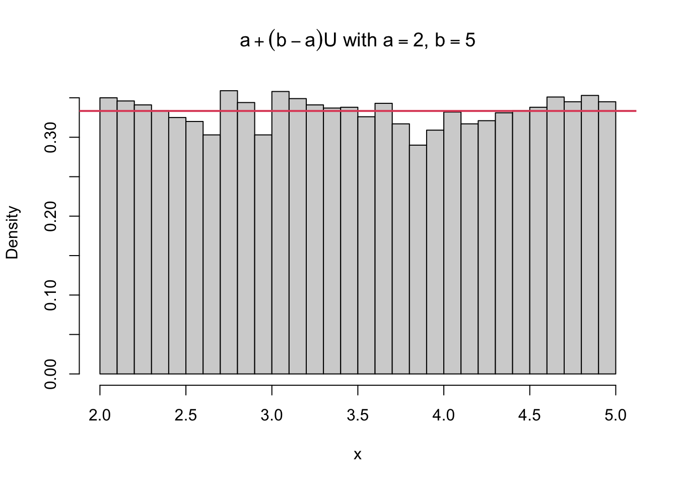
The simplest transformation of a uniform draw is a change of location and scale. If \(U \sim \mathrm{Unif}(0,1)\), then \(X = a + (b-a)\,U \sim \mathrm{Unif}(a,b)\), because

\[ P(X \le x) = P\!\left(U \le \frac{x-a}{b-a}\right) = \frac{x-a}{b-a}, \qquad a \le x \le b . \]

u <- runif(10000); x <- 2 + 3 * u          # Unif(2, 5)
hist(x, breaks = 30, freq = FALSE, main = TeX(r"($a + (b - a) U$ with $a = 2$, $b = 5$)"))
abline(h = 1/3, col = 2, lwd = 2)

Figure 4.2: Shows the simplest transformation of uniform random numbers, a change of location and scale. Histogram of \(10{,}000\) draws of \(2 + 3U\) with \(U \sim \mathrm{Unif}(0,1)\), against the \(\mathrm{Unif}(2, 5)\) density \(1/3\) (red).

4.1.4 Inverting the CDF

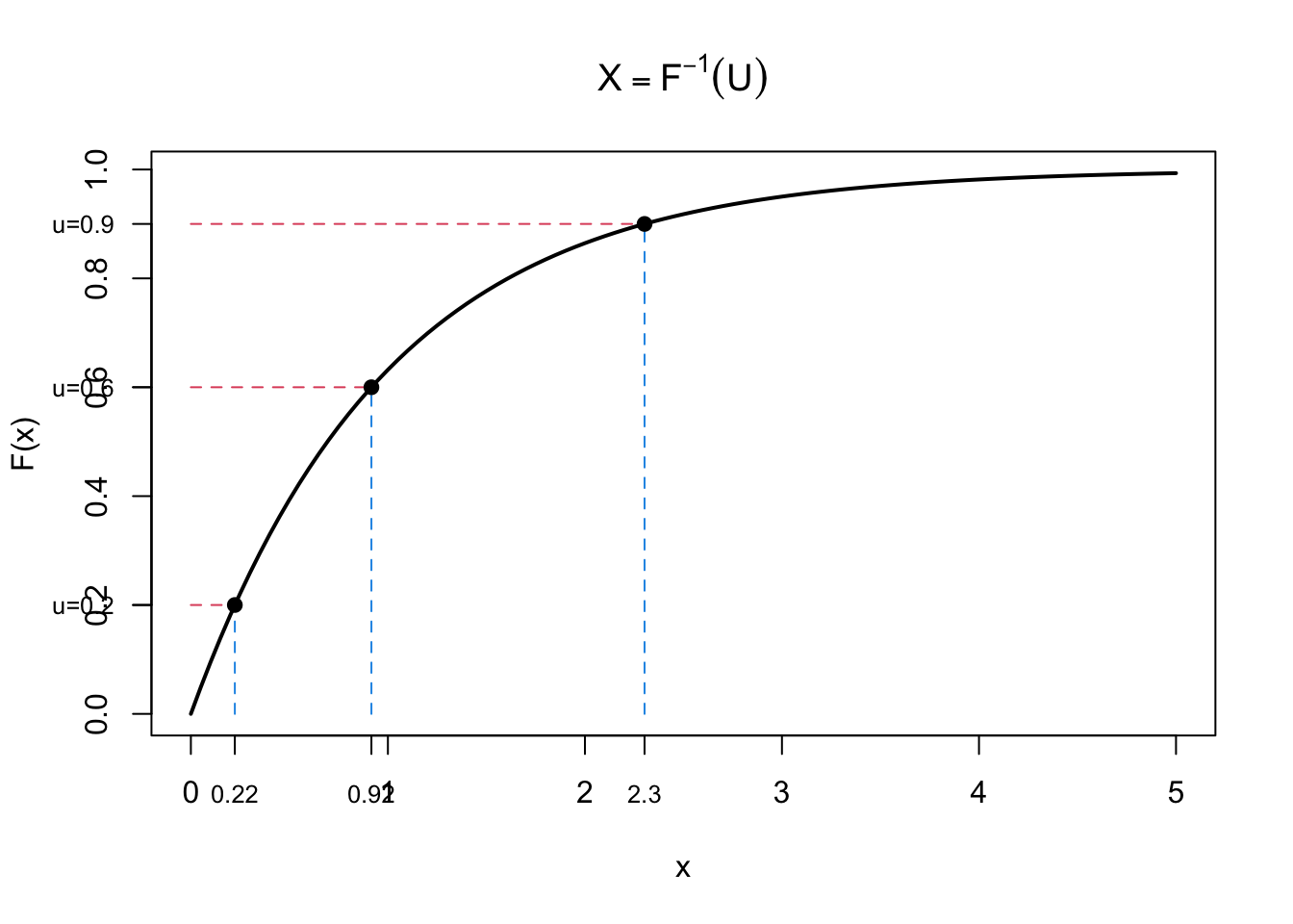
If we can generate \(U \sim \mathrm{Unif}(0,1)\), we can generate a random variable \(X\) from any continuous distribution using the inverse transform method. Let \(F_X\) be a continuous CDF with inverse (quantile function) \(F_X^{-1}\).

Theorem. If \(U \sim \mathrm{Unif}(0,1)\), then \(X = F_X^{-1}(U)\) has CDF \(F_X\).

Proof.

\[ P(X \le x) = P\big(F_X^{-1}(U) \le x\big) = P\big(U \le F_X(x)\big) = F_X(x). \]

Equivalently, by the change-of-variable formula with \(u = F_X(x)\),

\[ f_X(x) = f_U\big(F_X(x)\big)\left\lvert\frac{du}{dx}\right\rvert = 1 \times f(x). \]

The converse also holds: if \(X \sim F_X\), then \(F_X(X) \sim \mathrm{Unif}(0,1)\). This is the probability integral transform, which we will use for p-values in the section on hypothesis testing.

Figure 4.3: Shows geometrically how the inverse-CDF method turns uniform draws into draws from a target distribution. Three uniform values \(u\) on the vertical axis are mapped through the \(\mathrm{Exp}(1)\) CDF to \(x = F^{-1}(u)\) on the horizontal axis; where \(F\) is steep (high density), an interval of \(u\) values maps to a short interval of \(x\), so more draws land there.

4.1.5 Example: The Exponential Distribution

\(X \sim \mathrm{Exp}(\lambda)\) has CDF \(F_X(x) = 1 - e^{-\lambda x}\) for \(x > 0\). Setting \(u = 1 - e^{-\lambda x}\) and solving for \(x\) gives

\[ x = F_X^{-1}(u) = -\frac{1}{\lambda}\log(1-u). \]

Since \(1 - U \sim \mathrm{Unif}(0,1)\) as well, we may use \(X = -\log(U)/\lambda\).

lambda <- 2
u <- runif(10000)
x <- -log(u) / lambda
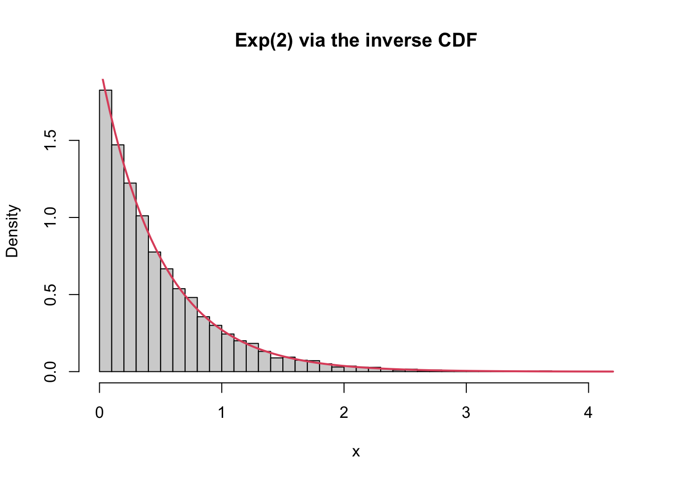
hist(x, breaks = 40, freq = FALSE, main = "Exp(2) via the inverse CDF")
curve(dexp(x, lambda), add = TRUE, col = 2, lwd = 2)
c(sample_mean = mean(x), true_mean = 1 / lambda)

sample_mean   true_mean 
  0.4989619   0.5000000 

Figure 4.4: Verifies the inverse-CDF method on a distribution whose inverse CDF has a closed form. Histogram of \(10{,}000\) draws of \(-\log(U)/\lambda\) with \(\lambda = 2\), against the \(\mathrm{Exp}(2)\) density (red).

4.1.6 Shinylive App for Inverse CDF Sampling

There is a shinylive app to demonstrate the inverse-CDF method for generating random numbers from a target distribution by transforming uniform draws.

4.1.7 A Special Transformation for Generating Normal Samples

The normal CDF \(\Phi\) has no closed-form inverse, so the inverse-CDF method is not directly usable. The Box–Muller transform instead generates pairs of independent standard normal variables from pairs of independent uniforms, by working in polar coordinates.

4.1.8 Two Standard Normals in Polar Coordinates

Write a pair \((Z_1, Z_2) \overset{iid}{\sim} N(0,1)\) in polar coordinates:

\[ Z_1 = R\cos\Theta, \qquad Z_2 = R\sin\Theta, \qquad R^2 = Z_1^2 + Z_2^2, \quad \Theta = \operatorname{atan2}(Z_2, Z_1). \]

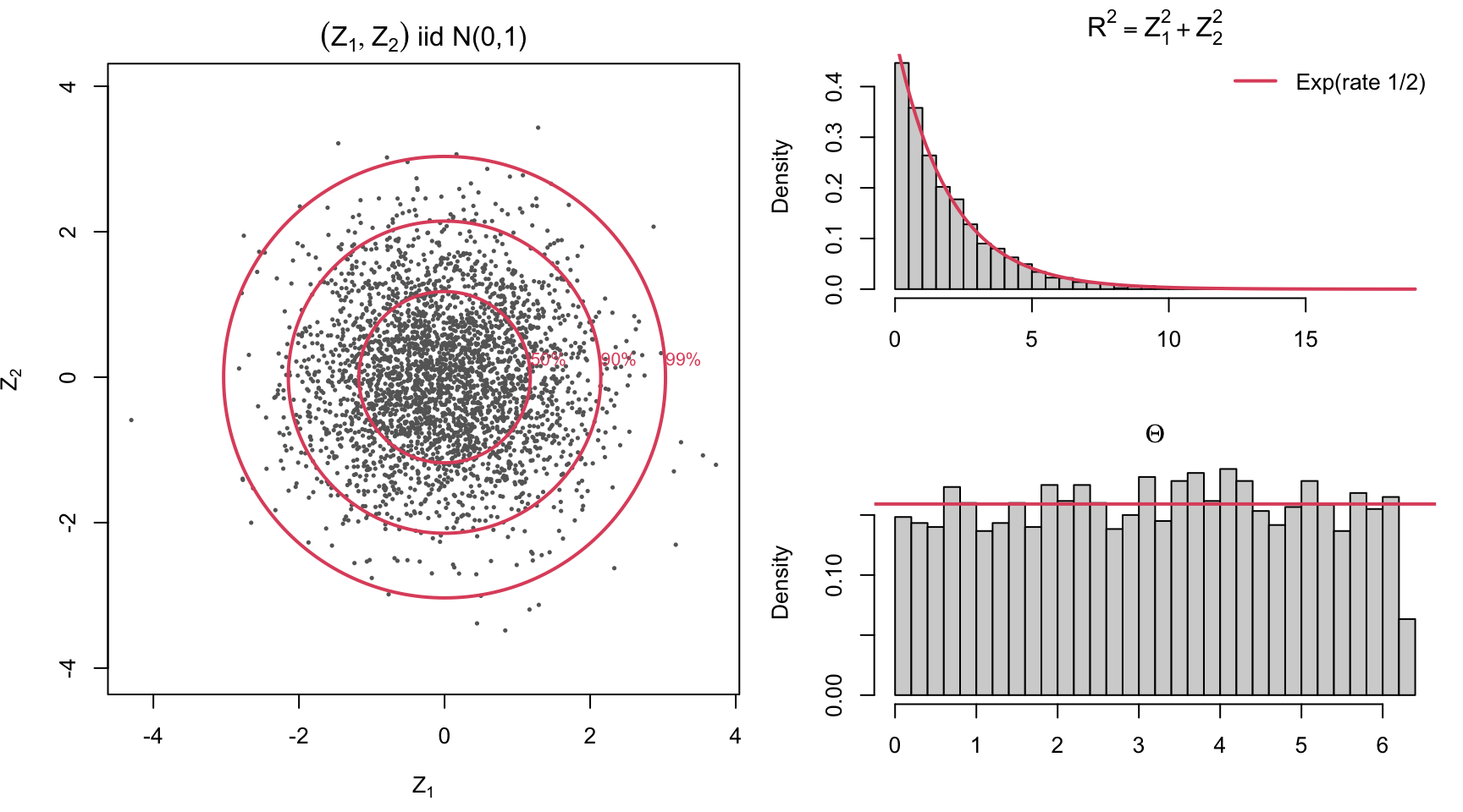
The joint density \(\frac{1}{2\pi}e^{-(z_1^2+z_2^2)/2}\) depends on \((z_1, z_2)\) only through \(r^2 = z_1^2 + z_2^2\), so it is rotationally symmetric about the origin. Consequently:

• The angle \(\Theta \sim \mathrm{Unif}(0, 2\pi)\), independently of \(R\).
• The squared radius \(R^2 = Z_1^2 + Z_2^2 \sim \chi^2_2\), and \(\chi^2_2\) is the exponential distribution with rate \(1/2\):

\[ f_{\chi^2_2}(w) = \frac{1}{2}e^{-w/2}, \quad w > 0 \qquad\Longrightarrow\qquad R^2 \sim \mathrm{Exp}(\text{rate} = 1/2). \]

Both \(R^2\) and \(\Theta\) can be generated by inverting a CDF.

Figure 4.5: Shows the two facts behind the Box-Muller transform: the angle of a pair of independent standard normals is uniform, and its squared radius is exponential. \(3000\) pairs \((Z_1, Z_2)\) of iid \(N(0,1)\) draws (left), with red circles enclosing 50%, 90% and 99% of the points; the squared radius \(R^2\) follows \(\mathrm{Exp}(1/2)\) (top right) and the angle \(\Theta\) is uniform on \((0, 2\pi)\) (bottom right).

4.1.9 The Box–Muller Transformation

Reversing the picture, we generate \(R^2\) and \(\Theta\) and then rotate back to \((Z_1, Z_2)\):

1. \(R^2 \sim \mathrm{Exp}(1/2)\) by the inverse CDF: \(F(w) = 1 - e^{-w/2}\), so \(R^2 = -2\log U_1\), that is, \(R = \sqrt{-2\log U_1}\).
2. \(\Theta \sim \mathrm{Unif}(0, 2\pi)\): \(\Theta = 2\pi U_2\).
3. \(Z_1 = R\cos\Theta\) and \(Z_2 = R\sin\Theta\).

Theorem (Box–Muller). If \(U_1, U_2 \overset{iid}{\sim} \mathrm{Unif}(0,1)\), then

\[ Z_1 = \sqrt{-2\log U_1}\,\cos(2\pi U_2), \qquad Z_2 = \sqrt{-2\log U_1}\,\sin(2\pi U_2) \]

are independent \(N(0,1)\) random variables. Two uniforms produce two normals, and \(\mu + \sigma Z \sim N(\mu, \sigma^2)\) then gives any normal distribution.

box_muller <- function(n) {
  u1 <- runif(n); u2 <- runif(n)
  r  <- sqrt(-2 * log(u1))            # R^2 ~ Exp(1/2), i.e. chi-square(2)
  th <- 2 * pi * u2                   # Theta ~ Unif(0, 2 pi)
  cbind(z1 = r * cos(th), z2 = r * sin(th))
}

z <- box_muller(500)
normal_sample <- c(z)                 # 1000 draws: both coordinates of 500 pairs

## R's built-in generator for comparison
nsample2 <- rnorm (1000)

par(mfrow=c(2,2),mar=c(4,4,2,1))
hist(normal_sample,main="Box-Muller Normal")
qqnorm(normal_sample, main="Box-Muller QQ")
qqline(normal_sample)
hist(nsample2, main="Built-in Normal")
qqnorm(nsample2, main="Built-in QQ")
qqline(nsample2)

c(mean = mean(z), sd = sd(z), corr = cor(z)[1, 2])

        mean           sd         corr 
 0.003366576  0.998441551 -0.000468918 

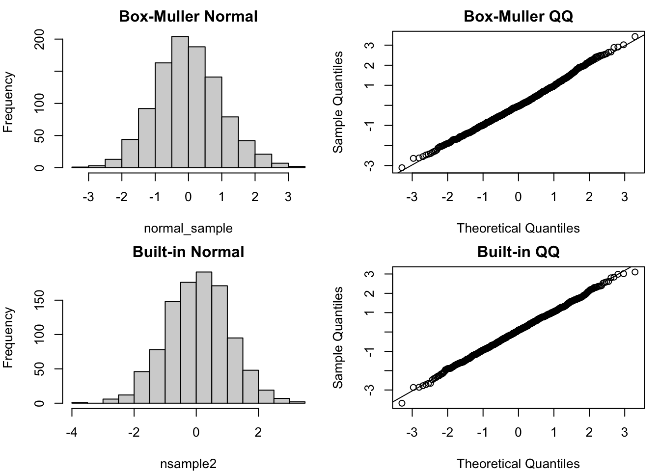
Figure 4.6: Shows how uniform random numbers can be transformed into normal ones, and verifies the Box-Muller construction against R’s rnorm(). Normal samples generated by the Box-Muller transform, compared with R’s built-in rnorm(): histogram and QQ plot for each.

The two coordinates have mean near 0, standard deviation near 1, and are uncorrelated, as the theorem asserts.

4.1.10 Law of Large Numbers and Central Limit Theorem

Monte Carlo estimates an expectation \(\mu = E(g(X))\) by an average of simulated values,

\[ \hat\mu_n = \frac{1}{n}\sum_{i=1}^n g(X_i), \qquad X_i \overset{iid}{\sim} f . \]

Two theorems justify this estimator and quantify its error.

Theorem (Strong Law of Large Numbers). If \(X_1, X_2, \ldots\) are iid with finite mean \(\mu\), then

\[ P\left(\frac{X_1 + \cdots + X_n}{n} \to \mu\right) = 1 . \]

The LLN guarantees that the average converges to the truth, but it does not say how fast.

Theorem (Central Limit Theorem). If, in addition, the variance \(\sigma^2\) is finite, then

\[ Z = \frac{\bar X_n - \mu}{\sigma/\sqrt n} \;\xrightarrow{d}\; N(0,1) \quad \text{as} \quad n \to \infty . \]

The CLT gives the error bound: the Monte Carlo error is of order \(\sigma/\sqrt n\).

4.1.11 Monte Carlo Error Bound from the CLT

By the CLT, with confidence level 95%,

\[ P\!\left(\lvert\bar X_n - \mu\rvert \le 1.96\,\frac{\sigma}{\sqrt n}\right) \approx 0.95, \]

so a 95% interval for \(\mu\) is

\[ \bar X_n \pm 1.96\,\frac{s}{\sqrt n}, \]

where the unknown \(\sigma\) is replaced by the sample standard deviation \(s\) of the simulated values.

• Halving the error requires four times as many samples, and each extra decimal digit of accuracy costs a 100-fold increase in \(n\).
• The rate \(n^{-1/2}\) does not depend on the dimension of \(X\), which is why Monte Carlo beats numerical quadrature in high dimensions.

4.1.12 Demonstrations

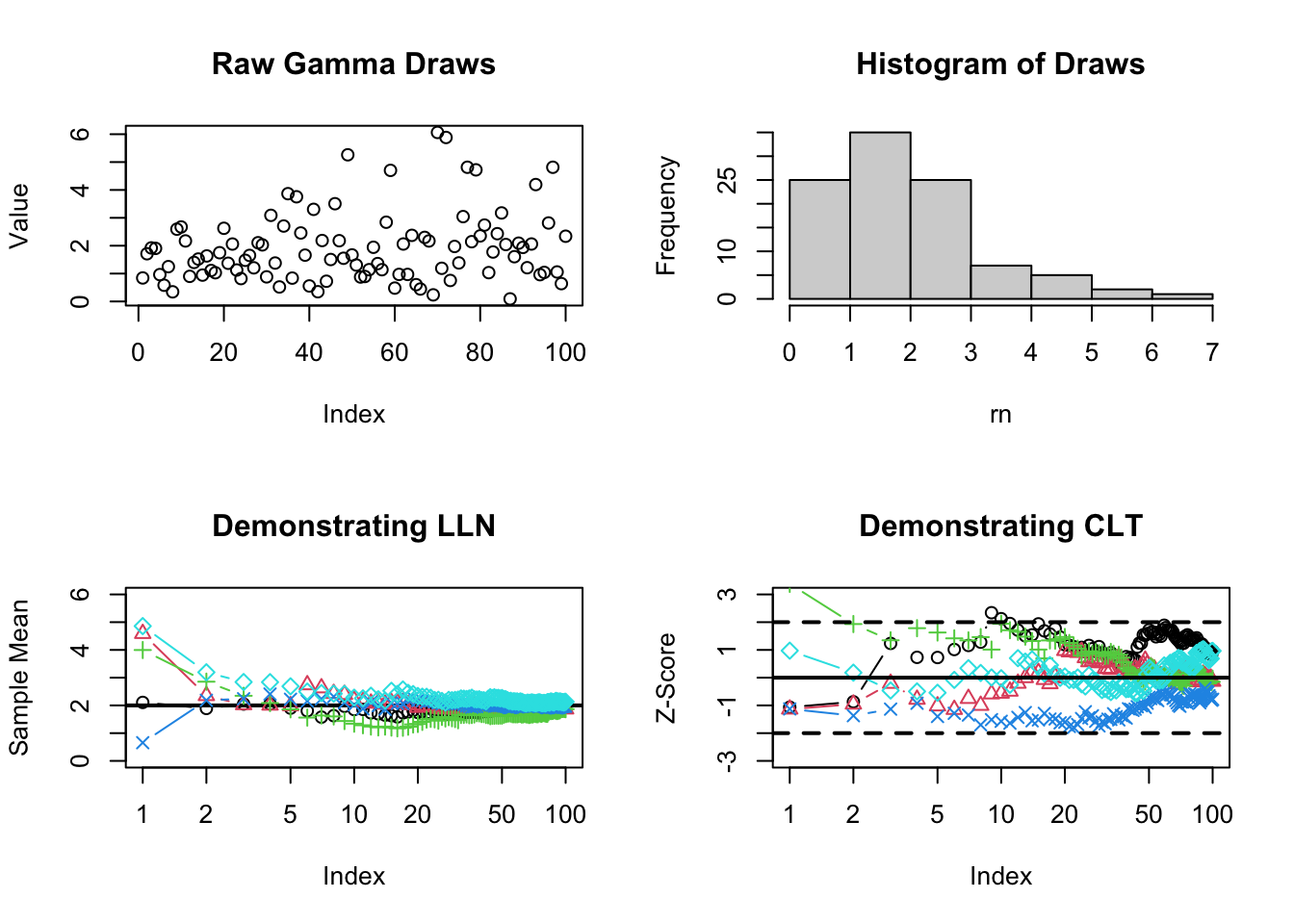
Here we draw from a Gamma distribution with shape parameter \(\alpha = 2\) and rate \(\beta = 1\). The theoretical mean is \(\mu = \alpha/\beta = 2\), and the variance is \(\sigma^2 = \alpha/\beta^2 = 2\).

n <- 100
rn <- rgamma(n, shape = 2)

par(mfrow = c(2,2))
plot(rn[1:100], main="Raw Gamma Draws", ylab="Value")
hist(rn, main="Histogram of Draws")

## Calculate running averages (LLN)
xbar.rep <- replicate(5, cumsum(rgamma(n, shape = 2))/(1:n))
## Calculate running standardized means (CLT)
se.rep <- replicate(5, (cumsum(rgamma(n, shape = 2))/(1:n) - 2) / sqrt(2/(1:n)))

## Plot LLN: should converge to mu = 2
plot(xbar.rep[,1], main = "Demonstrating LLN", log = "x", type = "b", ylim = c(0, 6), ylab="Sample Mean")
abline(h = 2, lwd=2)
for (i in 2:ncol(xbar.rep)) points(xbar.rep[,i], col = i, pch = i, type = "b")

## Plot CLT: should stabilize within roughly [-3, 3] standard deviations
plot(se.rep[,1], ylim = c(-3,3), type="b", log = "x", main="Demonstrating CLT", ylab="Z-Score")
for (i in 2:ncol(se.rep)) points(se.rep[,i], col = i, pch = i, type = "b")
abline(h = c(0, -2, 2), lty = c(1,2,2), lwd=2)

Figure 4.7: Illustrates the two theorems behind Monte Carlo methods: the Law of Large Numbers, under which averages converge to the mean, and the Central Limit Theorem, under which their fluctuations are approximately normal. Law of Large Numbers and Central Limit Theorem for the sample mean of Gamma(2,1) draws: raw draws, their histogram, running averages converging to \(\mu=2\), and standardized running means stabilizing to \(N(0,1)\).

The running standardized means in the last panel only show that \(Z\) stays on the \(N(0,1)\) scale. To see its distribution, we repeat the experiment \(N = 5000\) times: for each repetition we draw \(n\) values from the skewed \(\mathrm{Exp}(1)\) distribution and compute \((\bar X_n - 1)/(1/\sqrt n)\).

clt_demo <- function(n, N = 5000) replicate(N, (mean(rexp(n)) - 1) * sqrt(n))
par(mfrow = c(1, 3), mar = c(4, 4, 2, 1))
for (n in c(2, 10, 100)) {
  hist(clt_demo(n), breaks = 40, freq = FALSE, xlim = c(-4, 4),
       main = TeX(sprintf(r"($n = %d$)", n)), xlab = "")
  curve(dnorm, add = TRUE, col = 2, lwd = 2)
}

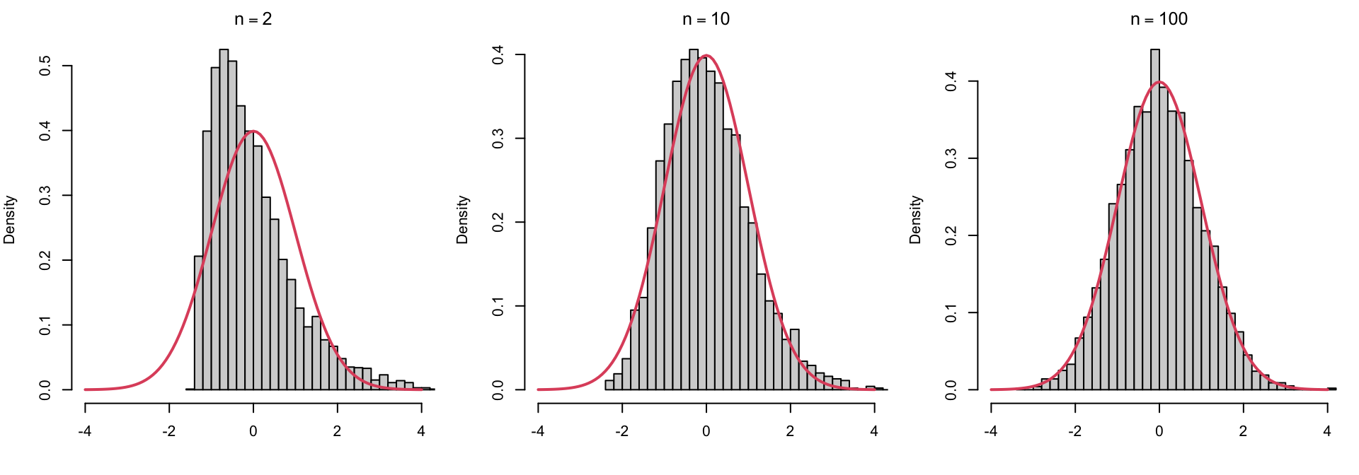
Figure 4.8: Shows the Central Limit Theorem as a statement about distributions: the standardized mean of skewed data becomes approximately normal as the sample size grows. Histograms of \(5000\) standardized means \((\bar X_n - 1)\sqrt n\) of \(\mathrm{Exp}(1)\) samples for \(n = 2, 10, 100\), against the \(N(0,1)\) density (red).

The skewness of the exponential is still visible at \(n = 2\) and \(n = 10\), and has almost disappeared at \(n = 100\).

4.1.13 An Example of Monte Carlo for Estimating \(\pi\)

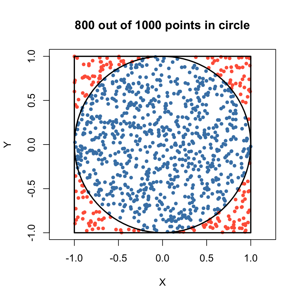
We can estimate the value of \(\pi\) by throwing random darts at a square with side length 2 (from \(-1\) to \(1\)) and counting how many land inside the inscribed circle of radius \(1\).

The area of the square is \((2)^2 = 4\), and the area of the circle is \(\pi(1)^2 = \pi\). Therefore, the probability that a uniform random point \((X,Y)\) falls inside the circle is: \[ P(X^2 + Y^2 \le 1) = \frac{\text{Area of Circle}}{\text{Area of Square}} = \frac{\pi}{4} \]

4.1.13.1 Visualizing the Method

Before we estimate \(\pi\), let’s visually simulate throwing 1,000 darts:

set.seed(123)
n_visual <- 1000
x_pts <- runif(n_visual, -1, 1)
y_pts <- runif(n_visual, -1, 1)
inside_circle <- (x_pts^2 + y_pts^2) <= 1

## Plot points
plot(x_pts, y_pts, col = ifelse(inside_circle, "steelblue", "tomato"),
     pch = 20, asp = 1, xlab = "X", ylab = "Y",
     main = paste(sum(inside_circle), "out of", n_visual, "points in circle"))

## Draw the boundaries
rect(-1, -1, 1, 1, border = "black", lwd = 2)
theta_seq <- seq(0, 2*pi, length.out = 100)
lines(cos(theta_seq), sin(theta_seq), col = "black", lwd = 2)

Figure 4.9: Illustrates Monte Carlo integration with a geometric example, estimating \(\pi\) as the proportion of random points that fall inside a circle. 1,000 uniform points (‘darts’) thrown at the \([-1,1]^2\) square; the fraction landing inside the inscribed circle gives a Monte Carlo estimate of \(\pi\).

4.1.13.2 The Monte Carlo Estimate

If we define an indicator variable \(I_i\) that equals 1 if the \(i\)-th dart lands in the circle and 0 otherwise, then \(E[I_i] = \pi/4\). We define \(Z_i = 4 \times I_i\), which gives \(E[Z_i] = \pi\) and

\[ \mathrm{Var}(Z_i) = 16 \cdot \frac{\pi}{4}\left(1 - \frac{\pi}{4}\right) \approx 2.70, \qquad \mathrm{SD}(Z_i) \approx 1.64 . \]

Our Monte Carlo estimate \(\hat{\pi}\) is the sample average of the \(Z_i\) values: \[ \hat{\pi} = \bar{Z} = \frac{1}{n}\sum_{i=1}^n Z_i = 4 \times \frac{\#\{i: X_i^2 + Y_i^2 \le 1\}}{n} \]

The Standard Error (SE) measures the uncertainty of our estimate. Using the sample standard deviation \(S_Z\), the 95% margin of error is calculated as: \[ \text{Margin of Error} = 1.96 \times \text{SE} = 1.96 \times \frac{S_Z}{\sqrt{n}} \]

The standard error is computed from the same simulated values as the estimate, at no extra cost, and should always be reported with a Monte Carlo estimate.

4.1.13.3 Results by Sample Size

We encapsulate the logic in a function and track how precision improves as \(n\) increases. The table below outlines our findings, including the actual error \(\hat\pi - \pi\) and the theoretical margin of error \(1.96 \times 1.64/\sqrt n\).

library(knitr)

## n is the number of samples drawn uniformly from the rectangle (-1,1)  * (-1,1)
## an estimate of pi is returned
pi_est_mc <- function(n)
{
    X <- runif(n,-1,1)
    Y <- runif(n,-1,1)

    # 4 times the indicator function
    Z <- 4 * (X^2 + Y^2 <= 1)

    mu <- mean(Z)
    error <- 1.96 * sd(Z) / sqrt(n)

    list(n = n, pi.est = mu, error.95perc = error, ci.lower = mu - error, ci.upper = mu + error)
}

## Run the estimation for varying sample sizes
sample_sizes <- c(100, 10000, 100000, 10000000)
results_list <- lapply(sample_sizes, pi_est_mc)

## Combine results into a dataframe for tabular display
results_df <- data.frame(
  N = sapply(results_list, function(x) x$n),
  Estimate = sapply(results_list, function(x) x$pi.est),
  Actual_Error = sapply(results_list, function(x) x$pi.est - pi),
  Error_Margin = sapply(results_list, function(x) x$error.95perc),
  Theory_Margin = 1.96 * 1.64 / sqrt(sample_sizes),
  CI_Lower = sapply(results_list, function(x) x$ci.lower),
  CI_Upper = sapply(results_list, function(x) x$ci.upper)
)

## Render the formatted table
kable(results_df,
      col.names = c("Sample Size (N)", "Estimated Pi", "Actual Error", "95% Margin of Error",
                    "Theoretical Margin", "Lower CI", "Upper CI"),
      digits = 6,
      caption = "Shows how the accuracy of the Monte Carlo estimate of $\\pi$, as measured by its margin of error, improves with the number of points. Monte Carlo Estimation of Pi across different sample sizes")

Table 4.1: Shows how the accuracy of the Monte Carlo estimate of \(\pi\), as measured by its margin of error, improves with the number of points. Monte Carlo estimation of pi across different sample sizes.

Shows how the accuracy of the Monte Carlo estimate of \(\pi\), as measured by its margin of error, improves with the number of points. Monte Carlo Estimation of Pi across different sample sizes

Sample Size (N)	Estimated Pi	Actual Error	95% Margin of Error	Theoretical Margin	Lower CI	Upper CI
1e+02	2.920000	-0.221593	0.349818	0.321440	2.570182	3.269818
1e+04	3.156400	0.014807	0.031985	0.032144	3.124415	3.188385
1e+05	3.143600	0.002007	0.010170	0.010165	3.133430	3.153770
1e+07	3.141769	0.000176	0.001018	0.001016	3.140751	3.142787

• The actual error is typically within the 95% margin of error, that is, within about 2 standard errors.
• The margin of error shrinks by a factor of \(\sqrt{k}\) when \(n\) grows \(k\)-fold (a factor of 10 for each 100-fold increase), as the CLT predicts, and agrees with its theoretical value.

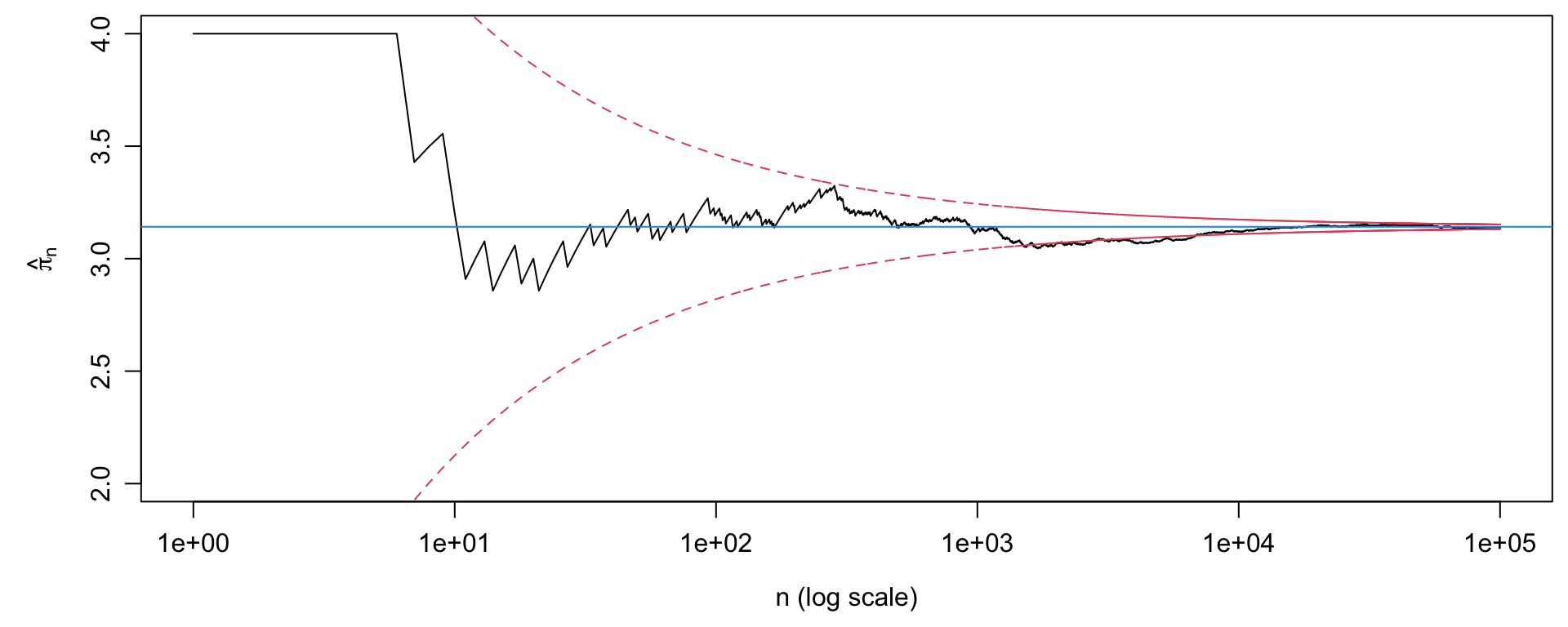
4.1.13.4 Convergence of \(\hat\pi_n\)

Following a single sequence of darts shows the same \(n^{-1/2}\) behaviour as it unfolds.

set.seed(1)
n <- 1e5; z <- 4 * (runif(n, -1, 1)^2 + runif(n, -1, 1)^2 <= 1)
k <- 1:n; pihat <- cumsum(z) / k
par(mar = c(4, 4.5, 0.5, 0.5), mgp = c(2.5, 0.8, 0))
plot(k, pihat, type = "l", log = "x", ylim = c(2, 4),
     xlab = "n (log scale)", ylab = expression(hat(pi)[n]))
lines(k, pi + 1.96 * 1.64 / sqrt(k), lty = 2, col = 2)
lines(k, pi - 1.96 * 1.64 / sqrt(k), lty = 2, col = 2)
abline(h = pi, col = 4)

Figure 4.10: Shows the Monte Carlo error bound at work along a single simulation run: the running estimate of \(\pi\) stays within a band that narrows at rate \(1/\sqrt{n}\). Running estimate \(\hat\pi_n\) over \(10^5\) darts (black), with the true value \(\pi\) (blue) and the band \(\pi \pm 1.96 \times 1.64/\sqrt n\) (red, dashed).

The running estimate stays inside the red band most of the time.

4.2 Point Estimation

Assume data \(X = (X_1, \ldots, X_n)\) is drawn from a distribution \(f(x; \theta)\) indexed by an unknown parameter \(\theta \in \Theta\). An estimator \(\hat\theta = T(X)\) is a function derived exclusively from the data. Because it relies on random samples, \(\hat\theta\) is itself a random variable. Its behavior is defined by its sampling distribution.

The two fundamental summaries of an estimator’s performance are bias and variance:

\[\mathrm{bias}(\hat\theta) = E_{\theta}(\hat\theta) - \theta, \qquad \mathrm{Var}_{\theta}(\hat\theta) = E_{\theta}\left[\left(\hat\theta - E_{\theta}(\hat\theta)\right)^{2}\right].\]

The most comprehensive single-number summary is the Mean Squared Error (MSE), defined as \(\mathrm{MSE}_{\theta}(\hat\theta) = E_{\theta}[(\hat\theta - \theta)^{2}]\). By adding and subtracting \(E_{\theta}(\hat\theta)\) inside the square, the cross term vanishes, yielding the MSE decomposition:

\[\mathrm{MSE}_{\theta}(\hat\theta) = \mathrm{Var}_{\theta}(\hat\theta) + \left[\mathrm{bias}_{\theta}(\hat\theta)\right]^{2}.\]

Key Insight: Unbiasedness is not strictly necessary. An estimator that introduces a small bias in exchange for a massive reduction in variance will frequently achieve a lower MSE than a strictly unbiased competitor.

Because MSE is a function of \(\theta\), it acts as the risk function under squared-error loss. Two estimators rarely have one absolute winner; their risk curves often cross. To choose a single estimator globally, statisticians summarize the risk curve via two main criteria:

• Minimax: Minimize the worst-case scenario: \(\sup_{\theta \in \Theta} \mathrm{MSE}_{\theta}(\hat\theta)\)
• Bayes Risk: Average the error against a prior distribution \(\pi\): \(\int_{\Theta} \mathrm{MSE}_{\theta}(\hat\theta)\, \pi(\theta)\, d\theta\)

Asymptotically, \(\hat\theta_n\) is consistent if it converges to \(\theta\) in probability. Under regularity conditions, Maximum Likelihood Estimators (MLEs) are consistent and asymptotically normal, achieving the Cramér–Rao lower variance bound \(1/I(\theta)\). However, in small samples, the MLE can often be outperformed.

4.2.1 Monte Carlo Evaluation of an Estimator

Risk functions are rarely available in closed form, but because they are expectations, we can estimate them efficiently using Monte Carlo simulation.

The Monte Carlo Recipe:

1. Define a grid of \(\theta\) values.
2. For each \(\theta\), generate \(N\) independent datasets \(X^{(j)} = (X_1^{(j)}, \ldots, X_n^{(j)})\), \(j = 1, \ldots, N\).
3. Compute the estimate \(\hat\theta^{(j)} = \hat\theta(X^{(j)})\) for each dataset.
4. Average the squared errors:

\[\widehat{\mathrm{MSE}}_{\theta} = \frac{1}{N} \sum_{j=1}^{N} \left(\hat\theta^{(j)} - \theta\right)^{2}\]

The bias and variance are estimated from the same replicates:

\[ \widehat{\mathrm{bias}}_{\theta} = \overline{\hat\theta} - \theta, \qquad \widehat{\mathrm{Var}}_{\theta} = \frac{1}{N}\sum_{j=1}^N \big(\hat\theta^{(j)} - \overline{\hat\theta}\big)^2, \qquad \overline{\hat\theta} = \frac{1}{N}\sum_{j=1}^N \hat\theta^{(j)} . \]

Two sample sizes appear: \(n\), the number of observations in each dataset, which is fixed by the problem; and \(N\), the number of replicates, which we choose large enough that the Monte Carlo error is negligible.

Because \(\widehat{\mathrm{MSE}}_{\theta}\) is an average of independent, identically distributed (i.i.d.) quantities, its standard error is \(s/\sqrt{N}\), where \(s^{2}\) is the sample variance of the squared errors. Always report the Monte Carlo error boundaries (\(\widehat{\mathrm{MSE}}_{\theta} \pm 1.96\, s/\sqrt{N}\)) to distinguish true differences in risk curves from mere simulation noise.

4.2.2 Example 1: Two Estimators of Proportions

Consider estimating a binomial proportion \(p\) from \(n\) independent trials.

• Maximum Likelihood Estimator (\(\hat{p}_1\)): The sample mean, \(\hat{p}_1 = \bar{X}\). This is unbiased but exhibits high variance in small samples, especially near boundaries (\(p \approx 0\) or \(1\)).
• Smoothed Estimator (\(\hat{p}_2\)): Often called the Laplace or “add-one-in” estimator, \(\hat{p}_2 = (\sum_i X_i + 1)/(n + 2)\). This introduces bias by shrinking the estimate toward \(1/2\) (the posterior mean under a uniform prior), but reduces variance by a factor of \([n/(n+2)]^2\).

We can estimate the risk curves on a grid of \(p\) values using the Monte Carlo method. Both estimators rely strictly on the sufficient statistic \(S = \sum_i X_i \sim \mathrm{Binomial}(n, p)\), allowing us to vectorize the simulation without looping over replicates.

###Estimators, written in terms of the sufficient statistic S = sum(X_i)
p_est1 <- function(s, n) s / n
p_est2 <- function(s, n) (s + 1) / (n + 2)

### Monte Carlo estimate of the MSE and its standard error.  All no_sim
### replicates are generated in a single vectorized draw.
mse_est_mc <- function(n, p, no_sim, p_est)
{
    sq_error <- (p_est(rbinom(no_sim, size = n, prob = p), n) - p)^2
    c(mse = mean(sq_error), sd = sqrt(var(sq_error) / no_sim))
}

### MSE over a grid of p values, returned as a 2 by length(p_set) matrix
mse_curve <- function(n, p_set, no_sim, p_est)
    vapply(p_set, function(p) mse_est_mc(n, p, no_sim, p_est), c(mse = 0, sd = 0))

no_sim <- 10000
p_set <- seq(0, 1, by = 0.05)
n_set <- c(2, 10, 50, 100)

par(mfrow = c(2, 2), mar = c(4, 4.5, 2.5, 1))

for (n in n_set)
{
    r1 <- mse_curve(n, p_set, no_sim, p_est1)
    r2 <- mse_curve(n, p_set, no_sim, p_est2)

    bands <- cbind(r1["mse", ], r1["mse", ] + 1.96 * r1["sd", ], r1["mse", ] - 1.96 * r1["sd", ],
                   r2["mse", ], r2["mse", ] + 1.96 * r2["sd", ], r2["mse", ] - 1.96 * r2["sd", ])

    matplot(p_set, bands, type = "l", lty = c(1, 2, 2, 1, 2, 2), col = rep(c(1, 2), each = 3),
            xlab = TeX(r"($p$)"),
            ylab = TeX(r"($E[(\hat{p} - p)^2]$)"),
            main = TeX(sprintf(r"($n = %d$)", n)))

    legend("top", bty = "n", lty = 1, col = c(1, 2), cex = 0.9,
           legend = TeX(c(r"($\hat{p}_1 = S/n$)", r"($\hat{p}_2 = (S+1)/(n+2)$)")))
}

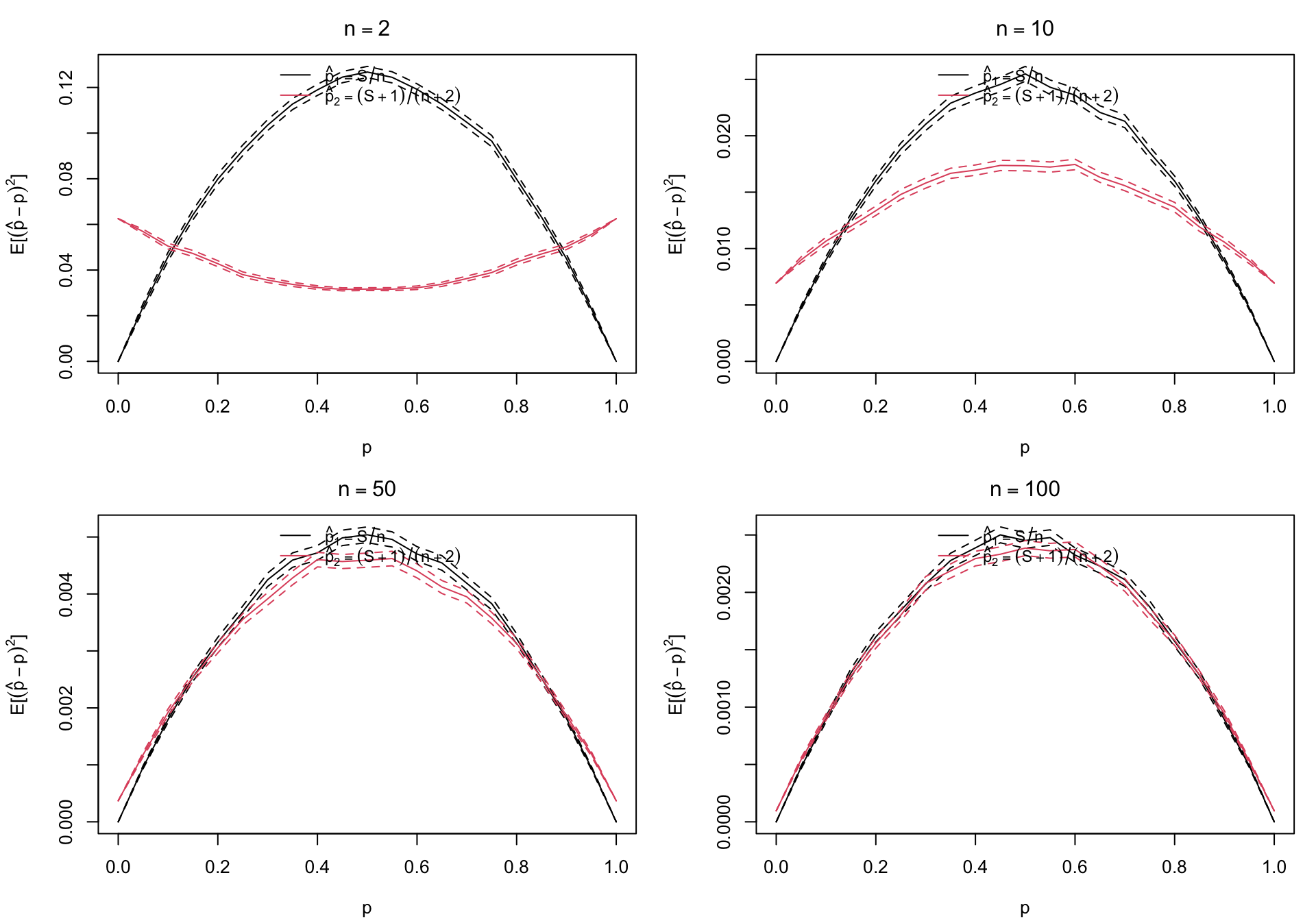
Figure 4.11: Uses simulation to compare two estimators of a binomial proportion by their mean squared error, showing when a small bias pays off through lower variance. Simulated MSE (with 95% Monte Carlo error bands) of \(\hat p_1 = S/n\) versus the smoothed \(\hat p_2 = (S+1)/(n+2)\), across \(n = 2, 10, 50, 100\).

When \(n\) is small, the smoothed estimator significantly outperforms the MLE across most of the parameter space. As \(n\) grows, the curves converge, reflecting the asymptotic efficiency of the MLE. The exception occurs strictly at the extremes (\(p \approx 0\) or \(1\)), where the shrinkage penalty overrides the variance reduction, making \(\hat{p}_1\) superior. The confidence bands confirm this crossing is a true mathematical property, not simulation variance.

4.2.3 Example 2: Mean, Median and Trimmed Mean

The choice between estimators can also depend on the shape of the data distribution rather than on the parameter value. Consider estimating the centre \(\theta = 0\) of a symmetric distribution from \(n = 20\) observations with three estimators: the sample mean, the sample median, and the 10% trimmed mean, which averages the observations after discarding the smallest and largest 10%. We estimate their bias, variance and MSE from \(N = 5000\) replicates, for normal data and for heavy-tailed \(t_3\) data.

eval_est <- function(rdist, n = 20, N = 5000) {
  est <- replicate(N, { x <- rdist(n); c(mean = mean(x), median = median(x), trim10 = mean(x, trim = 0.1)) })
  rbind(bias = rowMeans(est), var = apply(est, 1, var), mse = rowMeans(est^2))
}
kable(rbind(eval_est(rnorm),                          # normal data
            eval_est(function(n) rt(n, df = 3))),     # heavy-tailed t3 data
      digits = 4,
      col.names = c("mean", "median", "10% trimmed mean"),
      caption = "Monte Carlo bias, variance and MSE: normal data (rows 1-3) and $t_3$ data (rows 4-6).")

Table 4.2: Compares three estimators of the centre of a symmetric distribution under normal and heavy-tailed data, to show that the best estimator depends on the data distribution. Monte Carlo bias, variance and MSE of the mean, the median and the 10% trimmed mean, for \(n = 20\) observations from \(N(0,1)\) (top) and \(t_3\) (bottom), with \(N = 5000\) replicates.

Monte Carlo bias, variance and MSE: normal data (rows 1-3) and \(t_3\) data (rows 4-6).

	mean	median	10% trimmed mean
bias	-0.0033	-0.0028	-0.0026
var	0.0491	0.0730	0.0520
mse	0.0491	0.0730	0.0520
bias	-0.0039	-0.0025	-0.0031
var	0.1461	0.0871	0.0812
mse	0.1461	0.0871	0.0812

All three estimators are unbiased by symmetry, so the comparison is decided by the variance. No estimator is best everywhere: the mean wins under normality, where it is the MLE, while the trimmed mean and the median win under heavy tails, where a few extreme observations inflate the variance of the mean. The trimmed mean is a good compromise, losing little under normality.

4.3 Hypothesis Testing

A hypothesis test maps data to a binary decision about a null hypothesis \(H_0\) versus an alternative \(H_1\). It is built from a test statistic \(T\), whose large values are evidence against \(H_0\). This section shows that both the error rates of a test and, when the null distribution is unknown, the p-value itself are expectations, and so can be estimated by Monte Carlo.

4.3.1 The Two Types of Error

A test rejects \(H_0\) when the statistic \(T\) exceeds a critical value \(c_\alpha\). Crossing the decision with the truth gives four outcomes:

	reject: \(T > c_\alpha\)	do not reject: \(T \le c_\alpha\)
\(H_0\) true	Type I error (false positive)	true negative
\(H_1\) true	true positive	Type II error (false negative)

The two error rates of interest are the size and the power:

\[ \text{size} = P(T > c_\alpha \mid H_0) = \alpha, \qquad \text{power} = P(T > c_\alpha \mid H_1) = 1 - \beta . \]

When \(H_0\) is composite, the size is the largest type I error probability over all parameter values in \(H_0\), and a test has level \(\alpha\) if its size is at most \(\alpha\). Both size and power are probabilities, hence expectations of indicators, so both can be estimated by Monte Carlo once we can simulate data under \(H_0\) and under \(H_1\).

4.3.2 Estimating False and True Positive Rates by Monte Carlo

For a test that rejects when \(T > c\), simulate \(N\) data sets under \(H_0\) and \(N\) data sets under \(H_1\), and compute \(T\) on each:

replicate	\(T^{(j)}_{H_0}\)	\(I(T^{(j)}_{H_0} > c)\)	\(T^{(j)}_{H_1}\)	\(I(T^{(j)}_{H_1} > c)\)
1	\(T^{(1)}_{H_0}\)	0	\(T^{(1)}_{H_1}\)	1
2	\(T^{(2)}_{H_0}\)	1	\(T^{(2)}_{H_1}\)	1
\(\vdots\)	\(\vdots\)	\(\vdots\)	\(\vdots\)	\(\vdots\)
\(N\)	\(T^{(N)}_{H_0}\)	0	\(T^{(N)}_{H_1}\)	0

The false and true positive rates are estimated by the averages of the two indicator columns:

\[ \widehat{\text{FPR}}(c) = \frac{1}{N}\sum_{j=1}^N I\big(T^{(j)}_{H_0} > c\big), \qquad \widehat{\text{TPR}}(c) = \frac{1}{N}\sum_{j=1}^N I\big(T^{(j)}_{H_1} > c\big). \]

\(\widehat{\text{FPR}}\) estimates the size (the type I error rate) and \(\widehat{\text{TPR}}\) estimates the power, \(1 - \beta\). To obtain a test of size \(\alpha\) when the null distribution of \(T\) is unknown, take \(\hat c_\alpha\) to be the \((1-\alpha)\) sample quantile of \(T^{(1)}_{H_0}, \ldots, T^{(N)}_{H_0}\); this replaces the null distribution of \(T\) by its empirical distribution.

4.3.3 The p-value: A Probability Integral Transform of \(T\) under \(H_0\)

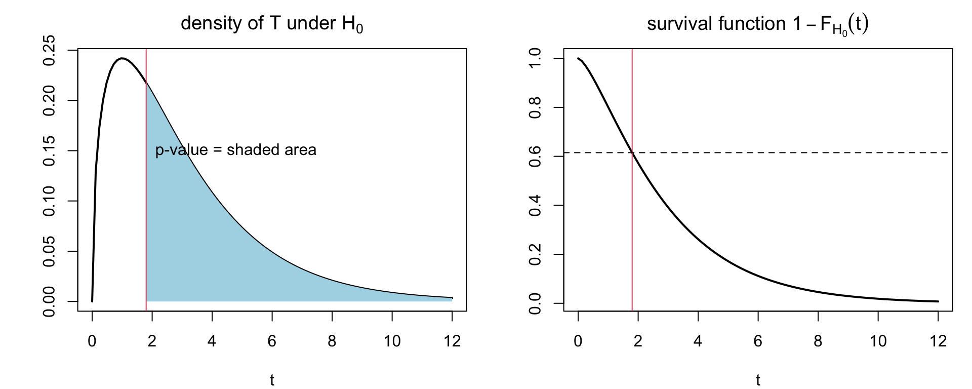
The p-value repackages the test so that no \(\alpha\) has to be fixed in advance. It is the probability, under \(H_0\), of a statistic at least as extreme as the observed one:

\[ \text{p-value}(t) = P(T \ge t \mid H_0) = 1 - F_{H_0}(t), \]

that is, the survival function of \(T\) under \(H_0\) evaluated at \(t^{obs}\). Rejecting when \(\text{p-value}(t^{obs}) < \alpha\) is the same as rejecting when \(t^{obs} > c_\alpha\).

par(mfrow = c(1, 2), mar = c(4, 4, 2.5, 1))
t0 <- 1.8
curve(dchisq(x, 3), 0, 12, lwd = 2, xlab = TeX(r"($t$)"), ylab = "",
      main = TeX(r"(density of $T$ under $H_0$)"))
xx <- seq(t0, 12, length = 100)
polygon(c(t0, xx, 12), c(0, dchisq(xx, 3), 0), col = "lightblue", border = NA)
abline(v = t0, col = 2)
text(t0 + 3, 0.15, "p-value = shaded area")
curve(1 - pchisq(x, 3), 0, 12, lwd = 2, xlab = TeX(r"($t$)"), ylab = "",
      main = TeX(r"(survival function $1 - F_{H_0}(t)$)"))
abline(v = t0, col = 2); abline(h = 1 - pchisq(t0, 3), lty = 2)

Figure 4.12: Shows that the p-value is a tail area of the null distribution of the test statistic, and equivalently the null survival function evaluated at the observed statistic. Left: the null density of \(T\) (here \(\chi^2_3\)) with the p-value of \(t^{obs} = 1.8\) shaded. Right: the survival function \(1 - F_{H_0}(t)\), whose height at \(t^{obs}\) is the same p-value.

4.3.4 Uniformity of the p-value under \(H_0\)

Theorem. If \(T \mid H_0\) has a continuous CDF \(F_{H_0}\), then \(\text{p-value}(T) = 1 - F_{H_0}(T) \sim \mathrm{Unif}(0,1)\) under \(H_0\).

Proof. For \(t \in (0,1)\),

\[ \begin{aligned} P\big(\text{p-value}(T) < t\big) &= P\big(1 - F_{H_0}(T) < t\big) = P\big(F_{H_0}(T) > 1 - t\big) \\ &= P\big(T > F_{H_0}^{-1}(1-t)\big) = 1 - F_{H_0}\big(F_{H_0}^{-1}(1-t)\big) = t . \end{aligned} \]

Two consequences follow.

• \(P(\text{p-value} < \alpha \mid H_0) = \alpha\) exactly, so rejecting when the p-value is below \(\alpha\) gives a test of size \(\alpha\).
• A histogram of p-values simulated under \(H_0\) should be flat. This is the standard test of a test: a histogram with excess mass near 0 means the test is liberal (its true size exceeds \(\alpha\)), and one with excess mass near 1 means it is conservative (it wastes power).

4.3.5 Monte Carlo Estimates of Size and Power

Simulating \(N\) data sets under \(H_0\) and \(N\) under \(H_1\) and computing the p-value of each, the size and power at level \(\alpha\) are estimated by the rejection rates

\[ \widehat{\text{size}} = \frac{1}{N}\sum_{j=1}^N I\big(\text{p-value}^{(j)}_{H_0} < \alpha\big), \qquad \widehat{\text{power}} = \frac{1}{N}\sum_{j=1}^N I\big(\text{p-value}^{(j)}_{H_1} < \alpha\big). \]

Each estimate is a proportion, so its Monte Carlo standard error is \(\sqrt{\hat p(1-\hat p)/N}\), about \(0.003\) for a size near \(0.05\) with \(N = 5000\).

Throughout this section, simulated p-values are displayed with the helper below. Its bins have width \(\alpha\), so the first bar (in red) holds exactly the rejected data sets, and the legend reports the rejection rate: the estimated size under \(H_0\), or the estimated power under \(H_1\).

hist_reject <- function(pv, main, alpha = 0.05) {
  br <- seq(0, 1, by = alpha)                  # first bar = rejection region
  ymax <- max(hist(pv, breaks = br, plot = FALSE)$counts)
  hist(pv, breaks = br, main = main, xlab = "p-value",
       ylim = c(0, 1.3 * ymax),                # headroom for the legend
       col = ifelse(br[-1] <= alpha, "red", "grey80"))
  abline(v = alpha, col = "red", lwd = 2, lty = 2)
  legend("topright", bty = "n", fill = c("red", NA), border = c("black", NA),
         lty = c(NA, 2), col = c(NA, "red"), lwd = c(NA, 2),
         legend = c(sprintf("rejected: %.3f", mean(pv < alpha)),
                    as.expression(bquote(alpha == .(alpha)))))
}

4.3.6 Example 1: The t-test under Different Data Settings

The one-sample \(t\)-test of \(H_0: \mu = 0\) assumes normally distributed observations. We first check it where that assumption holds, and then under heavy-tailed data, where it does not.

4.3.6.1 Normal Data

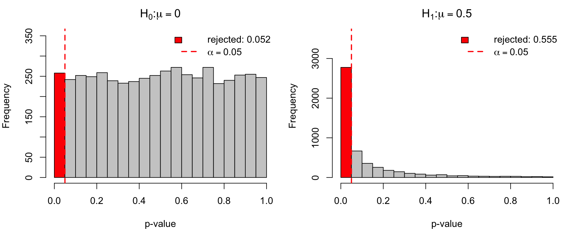
With \(n = 20\) normal observations and \(N = 5000\) simulated data sets, we compute the \(t\)-test p-value under \(H_0: \mu = 0\) and under \(H_1: \mu = 0.5\).

pv_sim <- function(mu, n = 20, N = 5000) replicate(N, t.test(rnorm(n, mu))$p.value)
pv0 <- pv_sim(0); pv1 <- pv_sim(0.5)

par(mfrow = c(1, 2), mar = c(4, 4, 2.5, 1))
hist_reject(pv0, TeX(r"($H_0: \mu = 0$)"))
hist_reject(pv1, TeX(r"($H_1: \mu = 0.5$)"))

c(size = mean(pv0 < 0.05), power = mean(pv1 < 0.05),
  exact_power = power.t.test(n = 20, delta = 0.5, sd = 1, type = "one.sample")$power)

       size       power exact_power 
  0.0516000   0.5552000   0.5644829 

Figure 4.13: Illustrates the basic simulation check of a test: p-values are uniform under the null hypothesis and concentrate near 0 under the alternative. p-values of the one-sample \(t\)-test for \(n = 20\) normal observations under \(H_0: \mu = 0\) (left) and \(H_1: \mu = 0.5\) (right); red bars are the rejections at \(\alpha = 0.05\).

Under \(H_0\) the p-values are uniform; under \(H_1\) they pile up near 0. The simulated power agrees with the exact power from power.t.test() to within Monte Carlo error.

4.3.6.2 Heavy-tailed Data: Null Distribution Diagnostics

We next simulate data from a \(t\)-distribution with \(\nu\) degrees of freedom. Smaller \(\nu\) gives heavier tails, and \(\nu = 1\) is the Cauchy distribution, which has no mean. The function below simulates N data sets of size n at once and returns their \(t\)-test p-values.

t.test.sim <- function (N, n, df, mu.true = 0, mu = 0)
{
    X <- matrix(rt(n * N, df), n, N) + mu.true
    m <- colMeans(X)
    v <- colSums((X - rep(m, each = n))^2) / (n - 1)
    2 * pt(-abs((m - mu) / sqrt(v / n)), n - 1)
}

t_main <- function (n, df, mu.true = 0)
    TeX(sprintf(r"($n = %d$, $\nu = %d$, $\mu = %g$)", n, df, mu.true))

N <- 2000

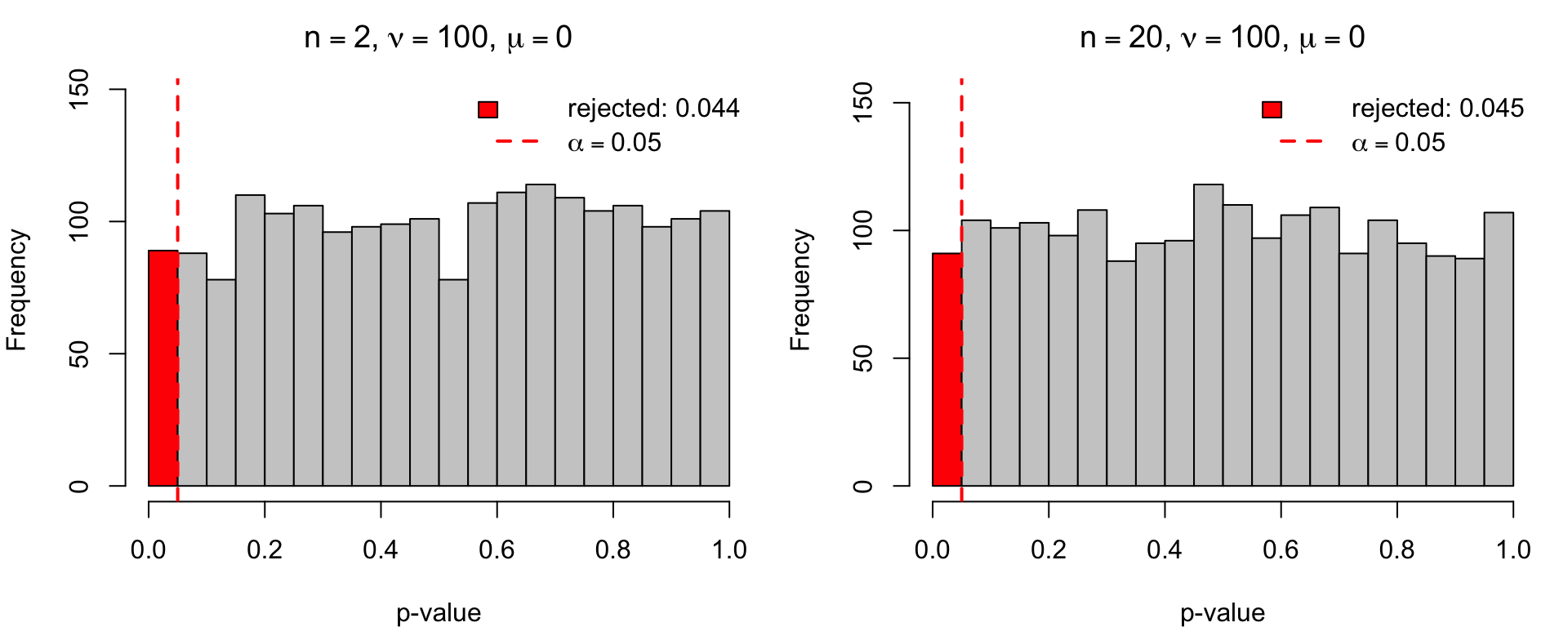
100 degrees of freedom (nearly normal). The data are practically normal, and the p-values are uniform for both \(n = 2\) and \(n = 20\).

par(mfrow = c(1, 2), mar = c(4, 4, 2.5, 1))
hist_reject(t.test.sim(N, 2, 100), t_main(2, 100))
hist_reject(t.test.sim(N, 20, 100), t_main(20, 100))

Figure 4.14: Uses simulation to check the size of the t-test: under the null hypothesis a valid test gives uniform p-values, and here the data are nearly normal. Null distribution of \(t\)-test p-values at \(\nu = 100\) (nearly normal), for \(n = 2\) and \(n = 20\): uniform, as expected.

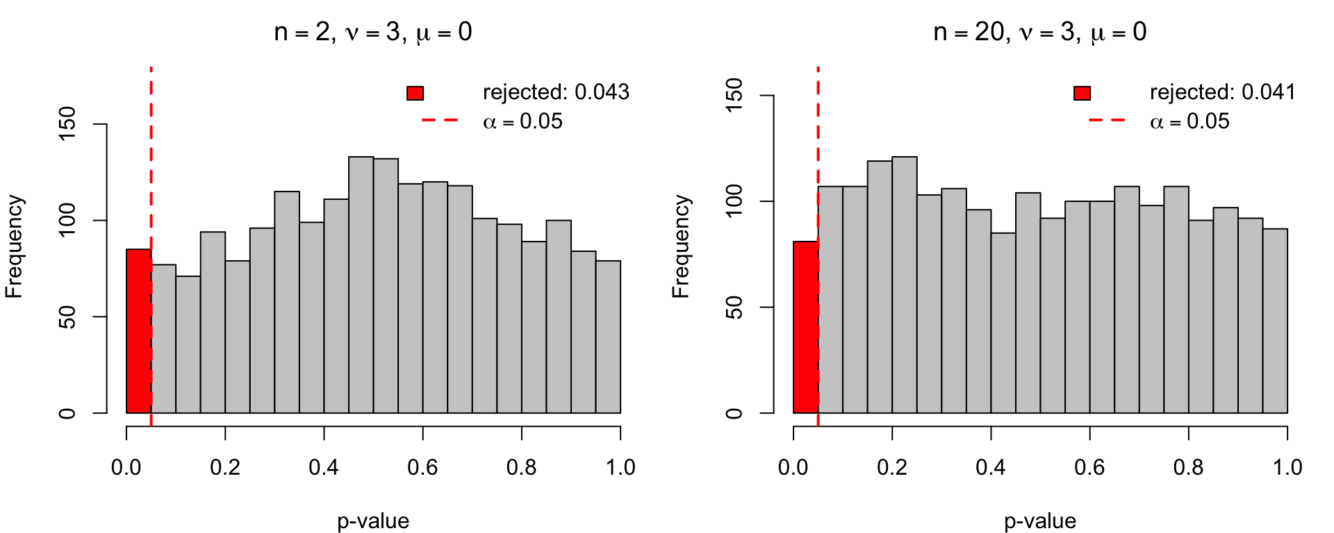
3 degrees of freedom (heavy tails). Heavier tails distort the p-value distribution, and the nominal type I error rate is no longer exactly calibrated.

par(mfrow = c(1, 2), mar = c(4, 4, 2.5, 1))
hist_reject(t.test.sim(N, 2, 3), t_main(2, 3))
hist_reject(t.test.sim(N, 20, 3), t_main(20, 3))

Figure 4.15: Repeats the size check of the t-test for heavy-tailed data to show how violating the normality assumption distorts the p-values. Null distribution of \(t\)-test p-values at \(\nu = 3\) (heavy tails), for \(n = 2\) and \(n = 20\): the tails pull the p-value distribution away from uniform.

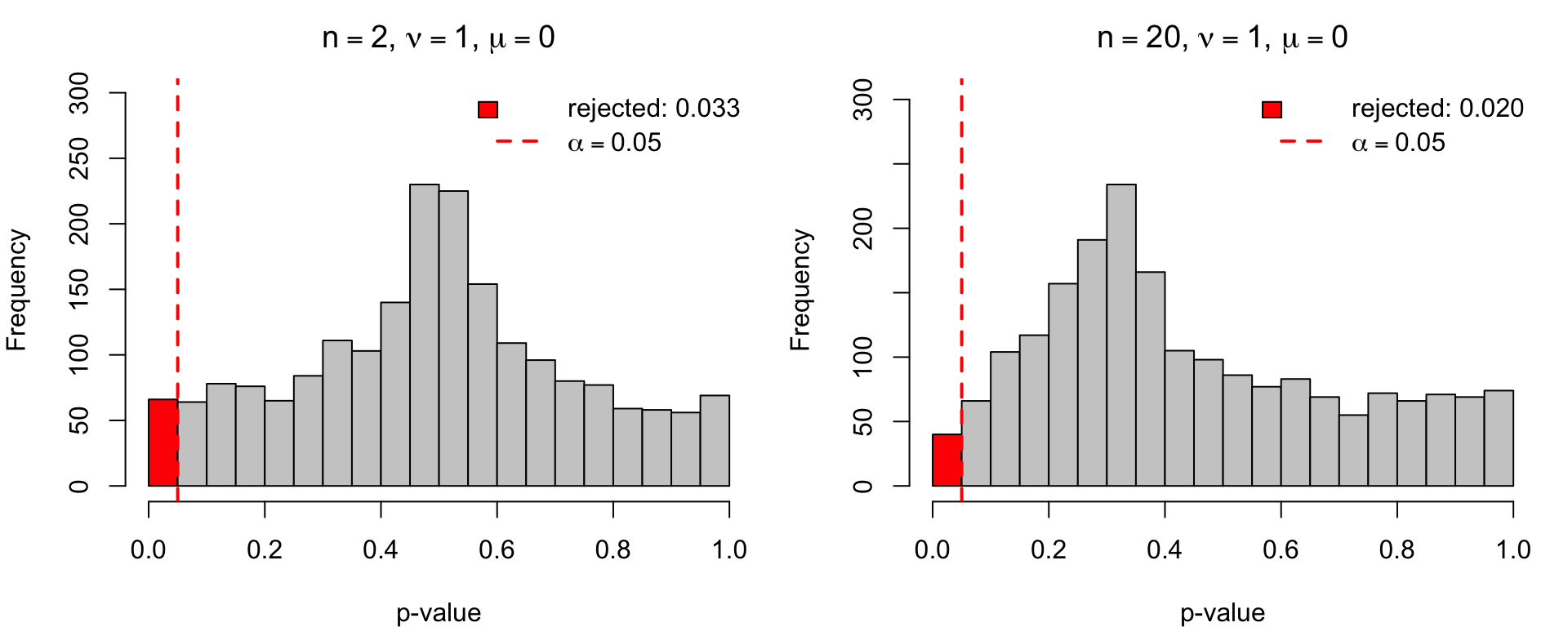
1 degree of freedom (Cauchy). With no finite mean or variance, a single extreme observation dominates both \(\bar X\) and \(s\), which pushes \(\lvert T\rvert\) toward 1 and the p-value toward the middle of \([0,1]\). The p-values are far from uniform and the rejection rate falls below \(\alpha\): the test is conservative, and it does not improve as \(n\) grows.

par(mfrow = c(1, 2), mar = c(4, 4, 2.5, 1))
hist_reject(t.test.sim(N, 2, 1), t_main(2, 1))
hist_reject(t.test.sim(N, 20, 1), t_main(20, 1))

Figure 4.16: Pushes the size check to the extreme case of Cauchy data, which have no mean, to show where the t-test breaks down completely. Null distribution of \(t\)-test p-values at \(\nu = 1\) (Cauchy), for \(n = 2\) and \(n = 20\): the p-values bunch in the middle of \([0,1]\) and the rejection rate is below 0.05.

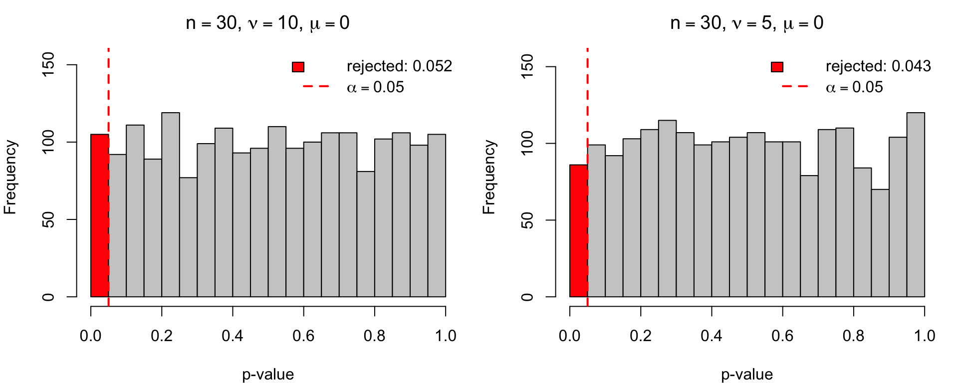
Larger sample size (\(n = 30\)). When the variance is finite, the Central Limit Theorem makes \(\bar X\) nearly normal as \(n\) grows, and the p-values for \(\nu = 10\) and \(\nu = 5\) are close to uniform again.

par(mfrow = c(1, 2), mar = c(4, 4, 2.5, 1))
hist_reject(t.test.sim(N, 30, 10), t_main(30, 10))
hist_reject(t.test.sim(N, 30, 5), t_main(30, 5))

Figure 4.17: Shows that a larger sample size can rescue the t-test for heavy-tailed data, because the Central Limit Theorem makes the sample mean nearly normal. Null distribution of \(t\)-test p-values at \(n = 30\) for \(\nu = 10\) and \(\nu = 5\): close to uniform even with heavy-tailed data.

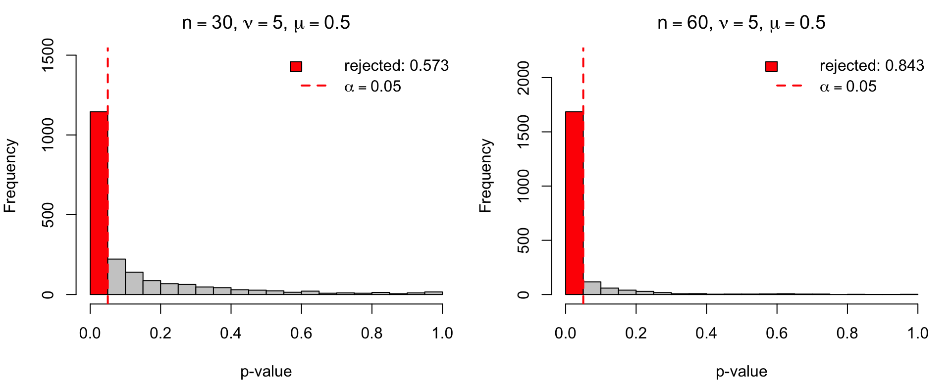
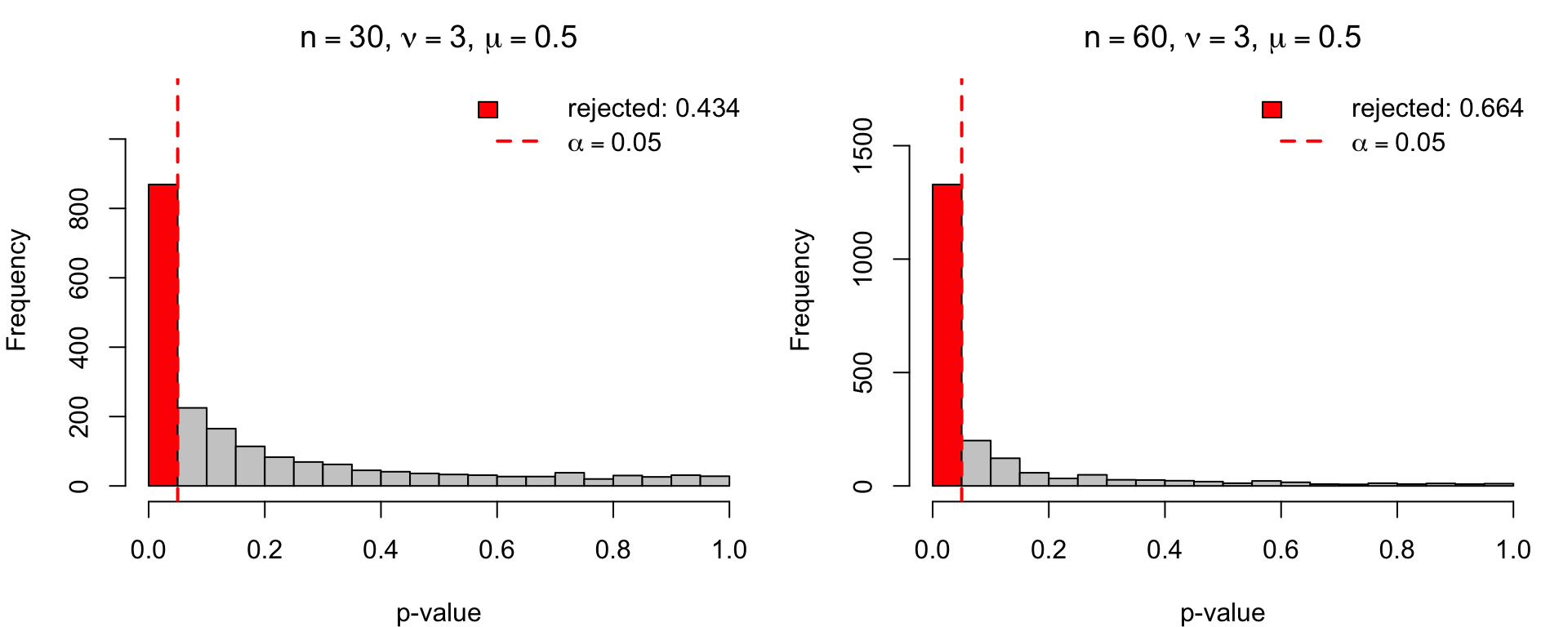
4.3.6.3 Heavy-tailed Data: Power

To estimate power, we shift the data to a true mean \(\mu = 0.5\) while still testing \(H_0: \mu = 0\). The rejection rate is now the power.

par(mfrow = c(1, 2), mar = c(4, 4, 2.5, 1))
hist_reject(t.test.sim(N, 30, 5, mu.true = 0.5), t_main(30, 5, 0.5))
hist_reject(t.test.sim(N, 60, 5, mu.true = 0.5), t_main(60, 5, 0.5))

Figure 4.18: Uses simulation to estimate the power of the t-test, its ability to detect a true mean of 0.5, when the data are moderately heavy-tailed. \(t\)-test p-values at \(\nu = 5\) with true mean \(\mu = 0.5\), for \(n = 30\) and \(n = 60\); the red rejection rate is the power.

par(mfrow = c(1, 2), mar = c(4, 4, 2.5, 1))
hist_reject(t.test.sim(N, 30, 3, mu.true = 0.5), t_main(30, 3, 0.5))
hist_reject(t.test.sim(N, 60, 3, mu.true = 0.5), t_main(60, 3, 0.5))

Figure 4.19: Repeats the power study for heavier-tailed data to show how tail weight affects the ability of the t-test to detect a real effect. \(t\)-test p-values at \(\nu = 3\) with true mean \(\mu = 0.5\), for \(n = 30\) and \(n = 60\); the red rejection rate is the power.

Heavier tails inflate the sample variance and so cost power; doubling \(n\) recovers much of it.

4.3.7 Monte Carlo for Calculating (Not Evaluating) a p-value

So far Monte Carlo has been used to evaluate a test whose p-value is known in closed form. When \(F_{H_0}\) is unknown, Monte Carlo can also calculate the p-value, by simulating \(T\) under \(H_0\):

\[ \widehat{\text{p-value}}(t^{obs}) = \frac{1 + \sum_{j=1}^N I\big(T^{(j)} \ge t^{obs}\big)}{N + 1}. \]

The “\(+1\)” counts the observed statistic as one draw from \(H_0\); it keeps the estimate above 0 and makes the test exactly valid for any finite \(N\).

As an example, we test \(H_0: \mu = 0\) for \(n = 15\) normal observations using \(T = \lvert\bar X\rvert/(s/\sqrt n)\), pretending that we do not know its \(t\)-distribution.

x <- rnorm(15, mean = 0.6); tobs <- abs(mean(x)) / (sd(x) / sqrt(15))
Tnull <- replicate(5000, { y <- rnorm(15); abs(mean(y)) / (sd(y) / sqrt(15)) })
c(mc_pv = (1 + sum(Tnull >= tobs)) / 5001, exact_pv = 2 * pt(-tobs, df = 14))

    mc_pv  exact_pv 
0.5278944 0.5319034 

This works only because the null hypothesis here fully specifies the distribution of the data. When it does not, as in a test of independence, a permutation test generates the null distribution from the data themselves.

4.3.8 Example 2: A Permutation Test for the Correlation Coefficient

4.3.8.1 Setting and Procedure

We observe pairs \((X_i, Y_i)\), \(i = 1, \ldots, n\), and test \(H_0: X \perp Y\) (which implies \(\mathrm{corr}(X,Y) = 0\)) with \(T = \lvert\hat\rho\rvert\). Under \(H_0\), every pairing of the \(X\) values with the \(Y\) values is equally likely, so the null distribution of \(T\) is obtained by re-computing \(T\) after randomly permuting \(Y\):

1. Compute \(\rho^{obs} = \hat\rho(X, Y)\).
2. For \(j = 1, \ldots, m\): permute \(Y\) to get \(Y^{(j)}\), and compute \(\rho^{(j)} = \hat\rho(X, Y^{(j)})\).
3. Compute \(\widehat{\text{p-value}} = \dfrac{1 + \# \{j : \lvert\rho^{(j)}\rvert \ge \lvert\rho^{obs}\rvert\}}{m+1}\).

No normality assumption is needed; the null distribution is generated from the data itself.

4.3.8.2 Replicated Data Sets by Permutation

\(X\) is held fixed, and each of the \(m\) permutations re-shuffles the \(Y\) column (shown for \(n = 5\)):

	\(X\)	observed \(Y\)	\(Y^{(1)}\)	\(Y^{(2)}\)	\(\cdots\)	\(Y^{(m)}\)
\(i = 1\)	\(x_1\)	\(y_1\)	\(y_3\)	\(y_5\)	\(\cdots\)	\(y_2\)
\(i = 2\)	\(x_2\)	\(y_2\)	\(y_1\)	\(y_4\)	\(\cdots\)	\(y_5\)
\(i = 3\)	\(x_3\)	\(y_3\)	\(y_5\)	\(y_1\)	\(\cdots\)	\(y_4\)
\(i = 4\)	\(x_4\)	\(y_4\)	\(y_2\)	\(y_3\)	\(\cdots\)	\(y_1\)
\(i = 5\)	\(x_5\)	\(y_5\)	\(y_4\)	\(y_2\)	\(\cdots\)	\(y_3\)
statistic		\(\rho^{obs}\)	\(\rho^{(1)}\)	\(\rho^{(2)}\)	\(\cdots\)	\(\rho^{(m)}\)
as extreme?			\(I(\lvert\rho^{(1)}\rvert \ge \lvert\rho^{obs}\rvert)\)	\(I(\lvert\rho^{(2)}\rvert \ge \lvert\rho^{obs}\rvert)\)	\(\cdots\)	\(I(\lvert\rho^{(m)}\rvert \ge \lvert\rho^{obs}\rvert)\)

\(\rho^{(1)}, \ldots, \rho^{(m)}\) are draws from the null distribution of \(\hat\rho\). The p-value is \(1\) plus the sum of the last row, divided by \(m + 1\).

4.3.8.3 Implementation in R

perm_cor_test <- function(x, y, m = 2000) {
  robs <- cor(x, y)
  rperm <- replicate(m, cor(x, sample(y)))
  list(rho = robs, pv = (1 + sum(abs(rperm) >= abs(robs))) / (m + 1), rperm = rperm)
}

4.3.8.4 Evaluation under \(H_0\) and \(H_1\)

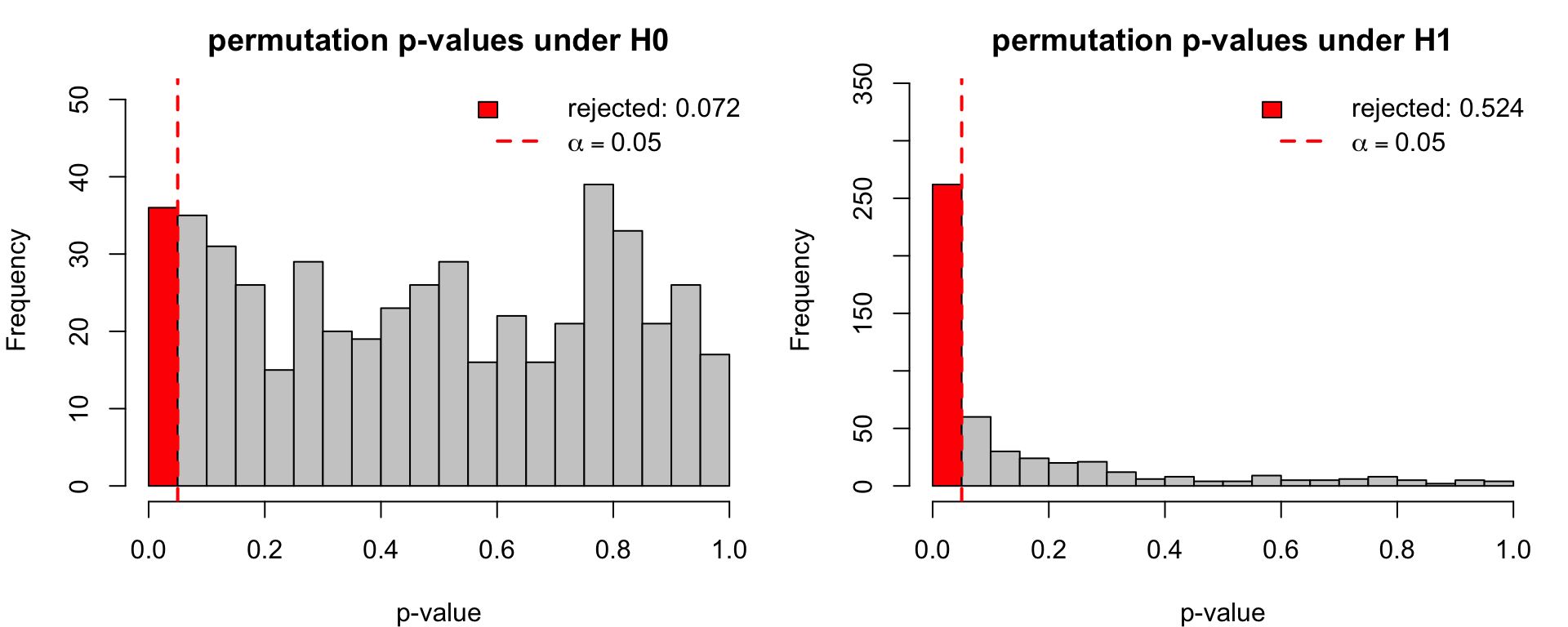
We generate non-normal \((X, Y)\): independent under \(H_0\), and \(Y = 0.4X + \epsilon\) under \(H_1\). We check that the permutation p-values are uniform with size \(\alpha\) under \(H_0\), and estimate the power under \(H_1\). Each of the \(N\) simulated data sets is analysed with its own complete permutation test:

data set	data under \(H_0\) (or \(H_1\))	\(\rho^{obs}\)	permutation test	p-value	reject?
\(k = 1\)	\((X^{[1]}, Y^{[1]})\)	\(\rho^{obs}_{1}\)	\(m\) permutations of \(Y^{[1]}\)	\(pv_1\)	\(I(pv_1 < \alpha)\)
\(k = 2\)	\((X^{[2]}, Y^{[2]})\)	\(\rho^{obs}_{2}\)	\(m\) permutations of \(Y^{[2]}\)	\(pv_2\)	\(I(pv_2 < \alpha)\)
\(\vdots\)	\(\vdots\)	\(\vdots\)	\(\vdots\)	\(\vdots\)	\(\vdots\)
\(k = N\)	\((X^{[N]}, Y^{[N]})\)	\(\rho^{obs}_{N}\)	\(m\) permutations of \(Y^{[N]}\)	\(pv_N\)	\(I(pv_N < \alpha)\)
summary				histogram	\(\widehat{\text{size}}\) (or \(\widehat{\text{power}}\)) \(= \frac{1}{N}\sum_k I(pv_k < \alpha)\)

Below, \(N = 500\) and \(m = 500\).

sim_cor <- function(n = 30, b = 0) { x <- rexp(n); list(x = x, y = b * x + rexp(n)) }
eval_perm_cor <- function(b, N = 500) replicate(N, {
  d <- sim_cor(b = b)
  perm_cor_test(d$x, d$y, m = 500)$pv
})
pv_cor0 <- eval_perm_cor(b = 0)      # H0: independent
pv_cor1 <- eval_perm_cor(b = 0.4)    # H1: dependent

par(mfrow = c(1, 2), mar = c(4, 4, 2.5, 1))
hist_reject(pv_cor0, "permutation p-values under H0")
hist_reject(pv_cor1, "permutation p-values under H1")

Figure 4.20: Verifies by simulation that the permutation test for correlation has the correct size without any normality assumption, and estimates its power. Permutation p-values for non-normal \((X, Y)\): independent under \(H_0\) (left), and \(Y = 0.4X + \epsilon\) under \(H_1\) (right); red bars are the rejections at \(\alpha = 0.05\).

Under \(H_0\) the permutation p-values are uniform on \([0,1]\) and the size is close to 0.05, with no distributional assumption on \((X, Y)\). Under \(H_1\) they pile up near 0, and the proportion below 0.05 is the power.

4.3.9 Example 3: Permuation Correction for Post-Selection Linear Regression

4.3.9.1 Setting

We have a response \(Y\) and \(p = 20\) candidate predictors \(X_1, \ldots, X_{20}\), with \(n = 50\), and want to test \(H_0\): \(Y\) is unrelated to all of the \(X\)’s. A common practice is to:

1. Pick the predictor \(X_{k^*}\) most correlated with \(Y\).
2. Fit \(Y \sim X_{k^*}\) and report the usual \(t\)-test p-value for its slope.

Is this a valid test of \(H_0\)? Does it have size \(\alpha\)?

test_lm_sel <- function(y, X) {
  k <- which.max(abs(cor(X, y)))
  summary(lm(y ~ X[, k]))$coefficients[2, 4]    # t-test p-value of selected slope
}

The \(t\)-test p-value assumes that \(X_{k^*}\) was chosen in advance. Selecting the best of 20 predictors after looking at the data means that, even under \(H_0\), \(\max_k \lvert\hat\rho_k\rvert\) tends to be large. The reported p-value ignores this selection.

4.3.9.2 Simulation for Evaluating test_lm_sel

We simulate \(N = 2000\) data sets with \(Y = \beta X_1 + \epsilon\): \(\beta = 0\) under \(H_0\), and \(\beta = 0.5\) under \(H_1\).

sim_lm <- function(n = 50, p = 20, beta = 0) {
  X <- matrix(rnorm(n * p), n, p); list(y = beta * X[, 1] + rnorm(n), X = X)
}
pv_sel0 <- replicate(2000, { d <- sim_lm(beta = 0);   test_lm_sel(d$y, d$X) })
pv_sel1 <- replicate(2000, { d <- sim_lm(beta = 0.5); test_lm_sel(d$y, d$X) })

par(mfrow = c(1, 2), mar = c(4, 4, 2.5, 1))
hist_reject(pv_sel0, "test_lm_sel p-values under H0")
hist_reject(pv_sel1, "test_lm_sel p-values under H1")

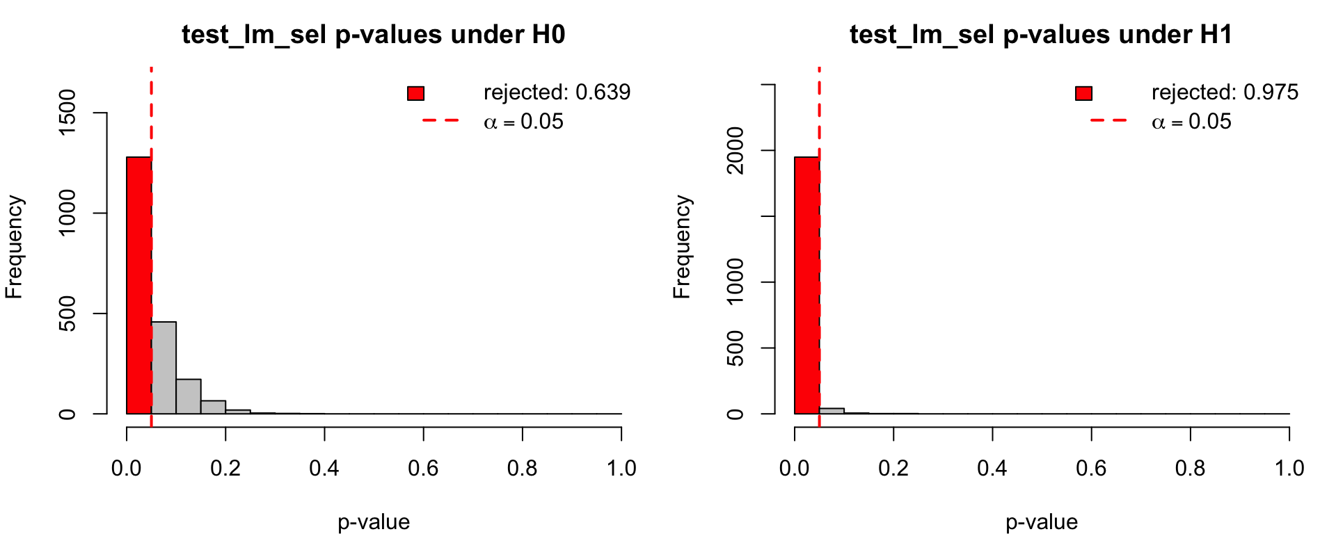
Figure 4.21: Demonstrates that choosing the best of many predictors using the data and then testing it as if it had been chosen in advance gives an invalid p-value. p-values of test_lm_sel under \(H_0\) (left) and \(H_1: \beta = 0.5\) (right); under \(H_0\) they are far from uniform, with a rejection rate far above 0.05.

The true size is far above 0.05: test_lm_sel rejects a true \(H_0\) far too often. Under \(H_0\) its p-value is not uniform, which is a general diagnostic for an invalid test. Its high rejection rate under \(H_1\) is not real power, since the test does not have size \(\alpha\).

4.3.9.3 The Permutation Fix

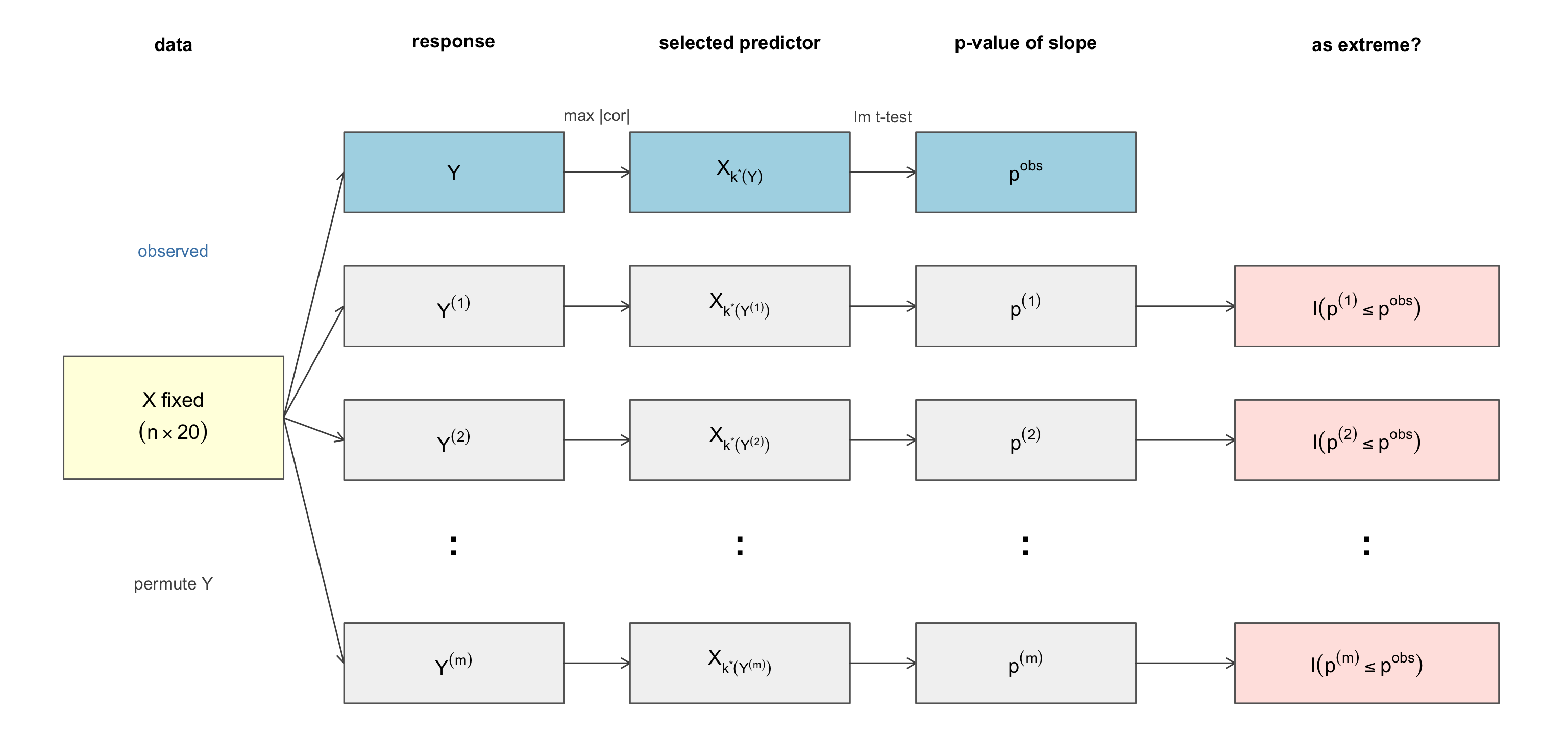
The fix is to repeat the whole procedure (select the most correlated variable, fit the linear model, report its p-value) on permuted responses, and to compare the observed p-value with the permutation distribution of p-values:

1. Compute \(p^{obs}\), the p-value of test_lm_sel on \((Y, X)\).
2. For \(j = 1, \ldots, m\): permute \(Y\), and compute \(p^{(j)}\), the p-value of test_lm_sel on \((Y^{(j)}, X)\), re-doing the selection each time.
3. Compute \(\widehat{\text{p-value}} = \dfrac{1 + \# \{j : p^{(j)} \le p^{obs}\}}{m+1}\), the proportion of permuted p-values at least as small as the observed one.

The selected index \(k^*(Y) = \arg\max_k \lvert\hat\rho(X_k, Y)\rvert\) is a function of the response, so each permuted \(Y^{(j)}\) gets its own selected predictor \(X_{k^*(Y^{(j)})}\), as Figure 4.22 shows.

par(mar = c(0, 0, 0, 0))
plot(NA, xlim = c(0, 13.2), ylim = c(0.2, 6.3), axes = FALSE, xlab = "", ylab = "")
box_at <- function(x, y, lab, col = "grey95", w = 1, h = 0.36) {
  rect(x - w, y - h, x + w, y + h, col = col, border = "grey40", lwd = 1.5)
  text(x, y, lab, cex = 1.25)
}
arr <- function(x0, y0, x1, y1) arrows(x0, y0, x1, y1, length = 0.1, lwd = 1.5, col = "grey30")
xs <- c(1.05, 3.6, 6.2, 8.8, 11.9)              # data, response, selection, p-value, compare
ys <- c(5, 3.8, 2.6, 1.55, 0.6)                 # branches: observed, 1, 2, ..., m
text(xs, 6.15, c("data", "response", "selected predictor", "p-value of slope", "as extreme?"),
     font = 2, cex = 1.15)
text(mean(xs[2:3]), 5.5, "max |cor|", cex = 1, col = "grey30")
text(mean(xs[3:4]), 5.5, "lm t-test", cex = 1, col = "grey30")
box_at(xs[1], 2.8, expression(atop(X ~ "fixed", (n %*% 20))), col = "lightyellow", h = 0.55)
resp <- list(quote(Y), quote(Y^(1)), quote(Y^(2)), NULL, quote(Y^(m)))
sel  <- list(quote(X[k^"*"*(Y)]), quote(X[k^"*"*(Y^(1))]), quote(X[k^"*"*(Y^(2))]), NULL,
             quote(X[k^"*"*(Y^(m))]))
pv   <- list(quote(p^obs), quote(p^(1)), quote(p^(2)), NULL, quote(p^(m)))
cmp  <- list(NULL, quote(I(p^(1) <= p^obs)), quote(I(p^(2) <= p^obs)), NULL, quote(I(p^(m) <= p^obs)))
for (b in c(1, 2, 3, 5)) {
  fill <- if (b == 1) "lightblue" else "grey95"
  arr(xs[1] + 1, 2.8, xs[2] - 1, ys[b])
  box_at(xs[2], ys[b], as.expression(resp[[b]]), col = fill)
  arr(xs[2] + 1, ys[b], xs[3] - 1, ys[b])
  box_at(xs[3], ys[b], as.expression(sel[[b]]), col = fill)
  arr(xs[3] + 1, ys[b], xs[4] - 1, ys[b])
  box_at(xs[4], ys[b], as.expression(pv[[b]]), col = fill)
  if (b > 1) {
    arr(xs[4] + 1, ys[b], xs[5] - 1.2, ys[b])
    box_at(xs[5], ys[b], as.expression(cmp[[b]]), col = "mistyrose", w = 1.2)
  }
}
text(xs[2:5], ys[4] + 0.1, ":", cex = 2.2, font = 2)
text(1.05, 4.3, "observed", col = "steelblue", cex = 1.05)
text(1.05, 1.3, "permute Y", col = "grey30", cex = 1.05)

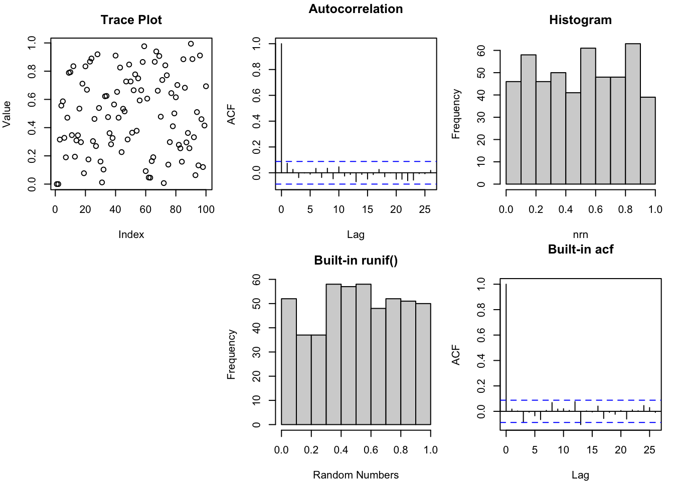
Figure 4.22: Shows why the selection step must be repeated inside the permutation loop: the selected predictor depends on the response, so every permuted response selects its own predictor. Tree of the permutation test after variable selection: the fixed \(X\) is paired with the observed \(Y\) and with each permuted \(Y^{(j)}\), each response selects its own predictor \(X_{k^*(Y^{(j)})}\), and the resulting slope p-value \(p^{(j)}\) is compared with \(p^{obs}\).

Keeping \(X_{k^*(Y)}\) fixed and only permuting \(Y\) would not reproduce the selection step, and the resulting test would still be invalid.

perm_lm_sel <- function(y, X, m = 500) {
  pobs <- test_lm_sel(y, X)
  pperm <- replicate(m, test_lm_sel(sample(y), X))
  (1 + sum(pperm <= pobs)) / (m + 1)
}

4.3.9.4 Evaluation under \(H_0\) and \(H_1\)

We simulate \((Y, X)\) from sim_lm, with \(\beta = 0\) under \(H_0\) and \(\beta = 0.5\) under \(H_1\), and run a complete permutation test on each data set:

data set	data under \(H_0\) (or \(H_1\))	\(p^{obs}\)	permutation test	p-value	reject?
\(k = 1\)	\((Y^{[1]}, X^{[1]})\)	\(p^{obs}_{1}\)	\(m\) permutations of \(Y^{[1]}\)	\(pv_1\)	\(I(pv_1 < \alpha)\)
\(k = 2\)	\((Y^{[2]}, X^{[2]})\)	\(p^{obs}_{2}\)	\(m\) permutations of \(Y^{[2]}\)	\(pv_2\)	\(I(pv_2 < \alpha)\)
\(\vdots\)	\(\vdots\)	\(\vdots\)	\(\vdots\)	\(\vdots\)	\(\vdots\)
\(k = N\)	\((Y^{[N]}, X^{[N]})\)	\(p^{obs}_{N}\)	\(m\) permutations of \(Y^{[N]}\)	\(pv_N\)	\(I(pv_N < \alpha)\)
summary				histogram	\(\widehat{\text{size}}\) (or \(\widehat{\text{power}}\)) \(= \frac{1}{N}\sum_k I(pv_k < \alpha)\)

Below, \(N = 300\) and \(m = 500\).

eval_perm_lm_sel <- function(beta, N = 300) replicate(N, {
  d <- sim_lm(beta = beta)
  perm_lm_sel(d$y, d$X, m = 500)
})
pv_perm0 <- eval_perm_lm_sel(beta = 0)      # H0: Y unrelated to X
pv_perm1 <- eval_perm_lm_sel(beta = 0.5)    # H1: Y depends on X1

par(mfrow = c(1, 2), mar = c(4, 4, 2.5, 1))
hist_reject(pv_perm0, "perm_lm_sel p-values under H0")
hist_reject(pv_perm1, "perm_lm_sel p-values under H1")

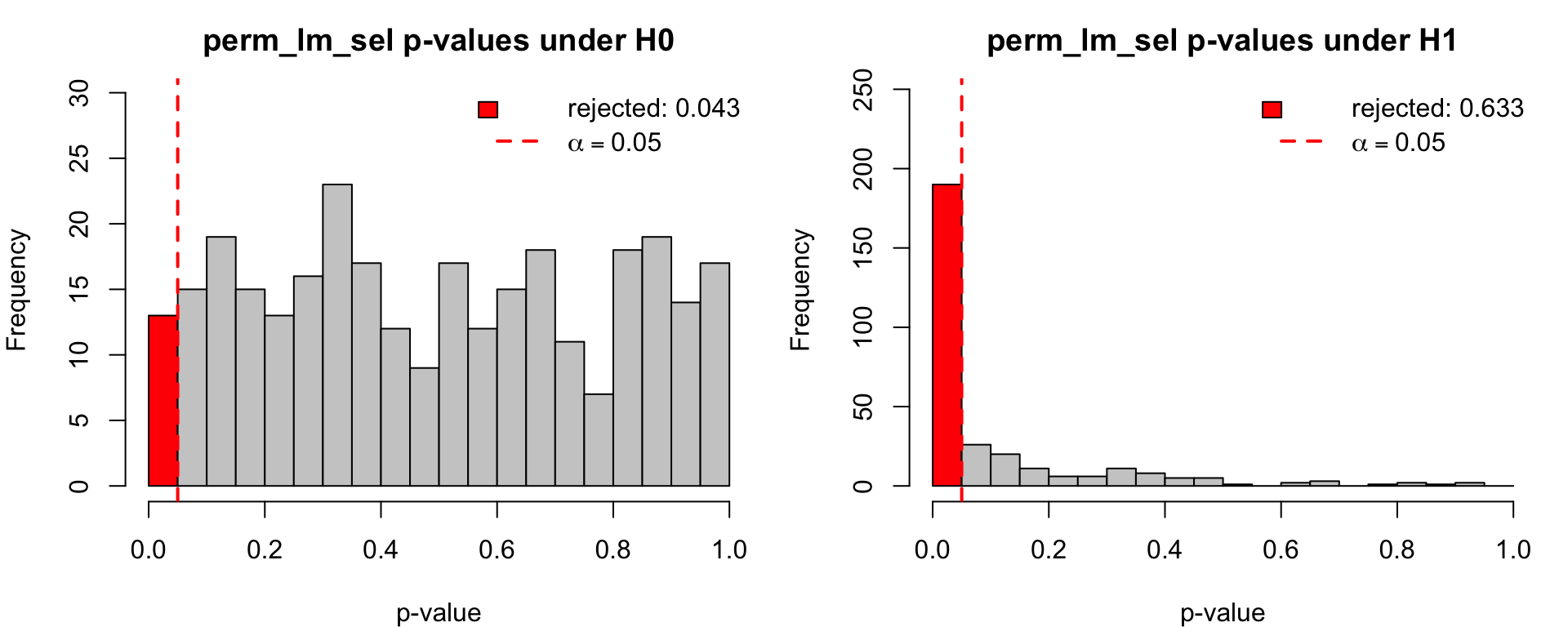
Figure 4.23: Shows that a permutation test which repeats the whole selection step on each shuffled data set restores valid p-values while keeping good power. Permutation p-values after variable selection under \(H_0\) (left) and \(H_1: \beta = 0.5\) (right): uniform with size near 0.05 under \(H_0\), and concentrated near 0 under \(H_1\).

Under \(H_0\) the permutation p-values are uniform and the size is close to 0.05; under \(H_1\) they pile up near 0, and the proportion below 0.05 is an honest power. The naive test rejects more often under \(H_1\) only because it also rejects far too often under \(H_0\): power comparisons are meaningful only between tests of the same size.

4.3.10 Advanced Computation-Intensive Tests

The examples above exposed two ways in which a textbook p-value can be biased:

1. A misspecified null distribution. The reference distribution is derived under assumptions (normality, known parameters, large samples) that the data do not satisfy, as for the \(t\)-test on heavy-tailed data.
2. A data-dependent procedure. The statistic is the result of a search (over predictors, models, thresholds or tuning parameters), but its p-value is computed as if the final choice had been fixed in advance, as for test_lm_sel.

Every method reviewed below corrects these biases with the same recipe: identify what is random under \(H_0\), re-generate data from \(H_0\) by simulation or resampling, re-run the entire procedure on each replicate, and read the p-value off the resulting reference distribution. The methods differ in how the null data are produced: by permutation when \(H_0\) is an exchangeability hypothesis, by a parametric bootstrap from a fitted null model when \(H_0\) leaves parameters unknown, and by resampling one variable given the others when \(H_0\) is a conditional independence hypothesis.

4.3.10.1 Monte Carlo Tests

The idea of computing a p-value by ranking the observed statistic among statistics simulated under \(H_0\) goes back to Barnard (1963) and was developed by Hope (1968). If \(T^{(1)}, \ldots, T^{(m)}\) are simulated under a simple null hypothesis, then under \(H_0\) the observed \(T\) is exchangeable with them, so

\[ \widehat{\text{p-value}} = \frac{1 + \#\{j : T^{(j)} \ge T^{obs}\}}{m + 1} \]

gives an exactly valid test for any \(m\), not just as \(m \to \infty\). Phipson and Smyth (2010) show that the tempting estimate \(\#\{j : T^{(j)} \ge T^{obs}\}/m\) can be zero and is anti-conservative, which matters most when many tests are corrected for multiplicity. Besag and Clifford (1989) extend Monte Carlo tests to nulls that can only be simulated by MCMC, and Besag and Clifford (1991) give a sequential version that stops simulating early once the p-value is clearly large, saving most of the computation for unremarkable data.

4.3.10.2 Parametric Bootstrap Tests with Estimated Parameters

Most null hypotheses are composite: they specify a family of distributions but not its parameters. Plugging estimated parameters into a reference distribution derived for known parameters biases the test. The classic example is the Kolmogorov–Smirnov (KS) test of normality with the mean and variance estimated from the data. The fitted normal is closer to the data than the true normal, so the KS distance is too small and the test is very conservative. Lilliefors (1967) tabulated the correct null distribution by Monte Carlo.

The general remedy is the parametric bootstrap test: fit the model under \(H_0\), simulate data sets from the fitted null model, re-estimate the parameters on each simulated data set, and recompute the statistic. For normality testing, the KS statistic of standardized data is location–scale invariant, so its null distribution does not depend on \((\mu, \sigma)\) at all, and simulating from \(N(0,1)\) gives an exact Monte Carlo test. Stute et al. (1993) establish the validity of this bootstrap for general goodness-of-fit tests with estimated parameters.

ks_stat <- function(x) {                       # KS distance to the fitted normal
  z <- sort((x - mean(x)) / sd(x)); n <- length(z); p <- pnorm(z)
  max(pmax((1:n) / n - p, p - (0:(n - 1)) / n))
}
ks_naive <- function(x)                        # pretends (mean, sd) were known
  suppressWarnings(ks.test(x, "pnorm", mean(x), sd(x))$p.value)
ks_mc <- function(x, m = 200) {                # re-estimates (mean, sd) on each null data set
  Dnull <- replicate(m, ks_stat(rnorm(length(x))))
  (1 + sum(Dnull >= ks_stat(x))) / (m + 1)
}

eval_ks <- function(rdata, N = 1000) replicate(N, {
  x <- rdata(); c(naive = ks_naive(x), mc = ks_mc(x))
})
ks_settings <- list("normal (H0)" = function() rnorm(50),
                    "t3 (H1)"     = function() rt(50, df = 3),
                    "exp (H1)"    = function() rexp(50))
ks_pv <- lapply(ks_settings, eval_ks)

par(mfrow = c(2, 3), mar = c(4, 4, 2.5, 1))
for (test in c("naive", "mc"))
  for (s in names(ks_pv))
    hist_reject(ks_pv[[s]][test, ], paste(test, "KS test:", s))

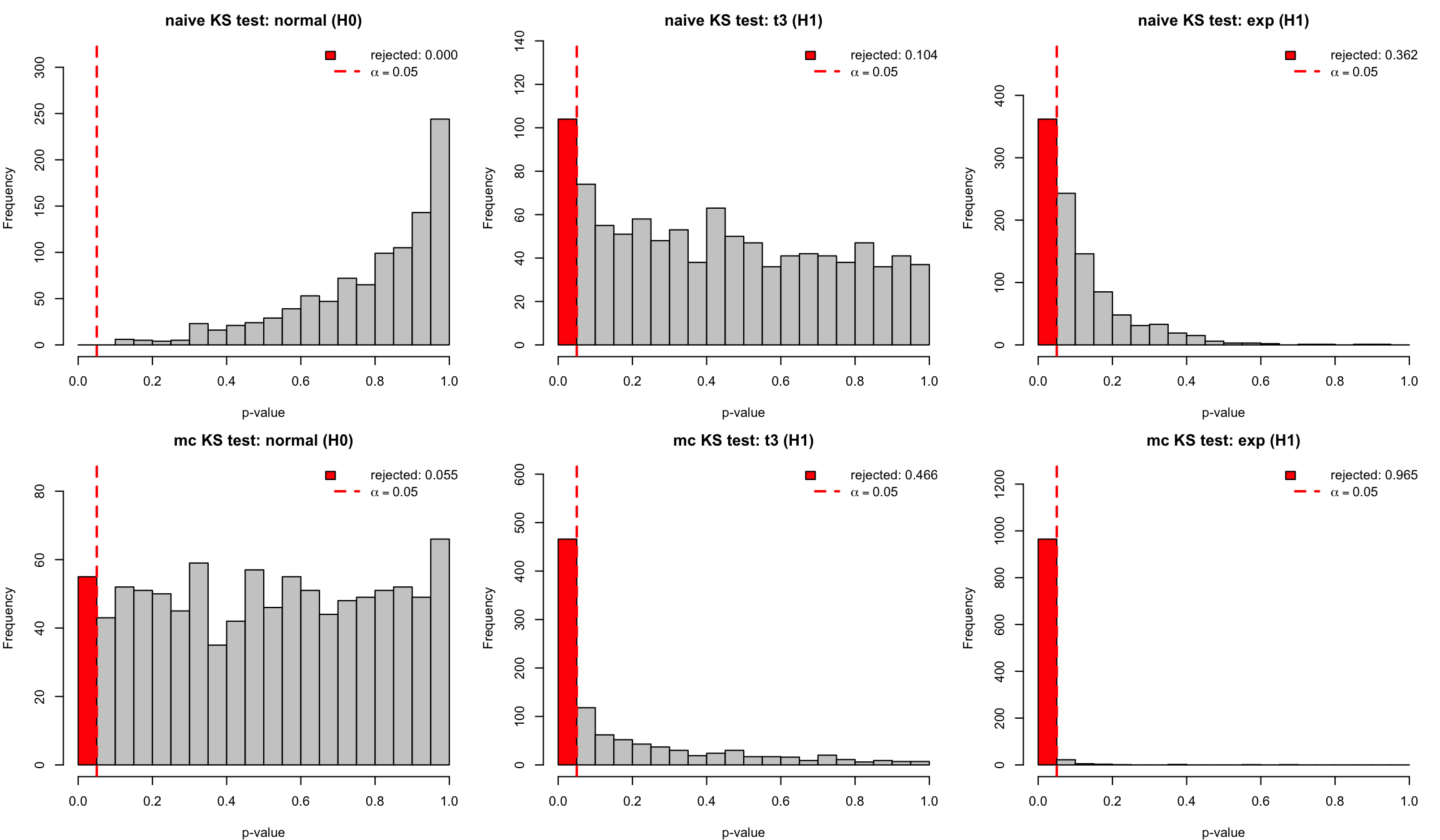
Figure 4.24: Shows how plugging estimated parameters into a textbook null distribution biases a goodness-of-fit test, and how a parametric bootstrap that re-estimates the parameters on every simulated data set removes the bias. p-values of the KS normality test with estimated mean and variance for \(n = 50\): the naive test (top) against the Monte Carlo test (bottom), for normal data (\(H_0\)), \(t_3\) data and exponential data; red bars are the rejections at \(\alpha = 0.05\).

Under \(H_0\) the naive p-values pile up near 1 and almost never reject, while the Monte Carlo p-values are uniform. Because the naive test is so conservative, it also has little power against both heavy-tailed and skewed alternatives. Correcting the size recovers most of that power.

Two guidelines from Hall and Wilson (1991) apply to every bootstrap test. First, resample from a distribution that satisfies \(H_0\) (for example, re-centre the data before resampling when testing a mean), not from the empirical distribution of the original data. Second, prefer an approximately pivotal statistic, such as a studentized one, whose null distribution depends little on the unknown parameters.

4.3.10.3 Maximum Statistics and Multiple Testing

The selection example is one instance of a general problem: the reported statistic is the maximum of many statistics, \(T_{\max} = \max_k T_k\), and each \(T_k\) is referred to its own marginal null distribution. Westfall and Young (1993) turned the permutation fix into a general method for multiple testing. Permuting the rows of the response jointly across all \(K\) hypotheses and recording \(\max_k T_k\) on each permutation gives adjusted p-values

\[ \tilde p_k = \frac{1 + \#\{j : \max_{l} T_l^{(j)} \ge T_k^{obs}\}}{m + 1}, \]

which control the family-wise error rate. Unlike the Bonferroni correction, the maxT (and the analogous minP) procedure automatically accounts for the correlation among the \(T_k\), and so is less conservative when the tests are dependent, as with nearby genes, voxels or genetic markers.

Scan statistics follow the same pattern with a search over locations. The spatial scan statistic of Kulldorff (1997) maximizes a likelihood ratio over many circular windows to find a disease cluster, and obtains its p-value by Monte Carlo replication of the whole search under a null of no clustering.

4.3.10.4 Nuisance Parameters Identified Only under the Alternative

In some problems the search is over a parameter that has no meaning under \(H_0\). Examples are the unknown date of a structural break in a regression, the threshold of a threshold autoregression, and the location of an extra component in a mixture model. Davies (1977) showed that the natural statistic is then a supremum over the unidentified parameter, and that it does not have the usual \(\chi^2\) distribution. Andrews (1993) derived the asymptotic null distribution of the sup-Wald (sup-\(F\)) test for a change point at an unknown date. Because that distribution depends on the design, Hansen (1996) proposed obtaining p-values by simulation.

Testing the number of components of a mixture is a related case in which the regularity conditions for the likelihood ratio test fail because the null lies on the boundary of the parameter space. McLachlan (1987) proposed calibrating the likelihood ratio statistic by a parametric bootstrap. Data sets are simulated from the fitted \(g\)-component model, and both the \(g\)- and \((g+1)\)-component models are refitted on each one, since the maximization over the extra component is exactly the search that biases the naive \(\chi^2\) reference.

4.3.10.5 Calibrating Asymptotic Tests: The Double Bootstrap

A test based on an asymptotic reference distribution has a level error that shrinks only slowly with \(n\). Beran (1988) proposed prepivoting: transform the statistic by its own estimated (bootstrap) null CDF, which makes it closer to pivotal and reduces the level error. Iterating the idea gives the double bootstrap. The p-value \(\hat p\) is computed by an inner bootstrap, and an outer bootstrap estimates the distribution of \(\hat p\) under the fitted null model. The corrected p-value is \(\Pr^*(\hat p^* \le \hat p)\), which is exactly the “p-value of a p-value” idea behind the permutation fix for variable selection. The cost is about \(B_1 \times B_2\) model fits; Davison and Hinkley (1997) discuss the implementation and when the extra accuracy is worth it.

4.3.10.6 Conditional Randomization Tests

Permuting a response tests marginal independence. In regression we usually want to test whether \(X_k\) is associated with \(Y\) given the other covariates \(X_{-k}\), which cannot be done by simply permuting \(X_k\) when the covariates are correlated. The conditional randomization test of Candès et al. (2018) assumes the distribution of \(X_k \mid X_{-k}\) is known or well estimated. It re-draws \(X_k^{(j)}\) from that conditional distribution, recomputes any test statistic (for example, the absolute lasso coefficient of \(X_k\), with the tuning parameter re-selected each time), and ranks the observed statistic among the simulated ones. The p-value is exactly valid for any statistic, however it was tuned, as long as the whole fitting procedure is repeated on every draw. The model-X knockoffs in the same paper replace the \(m\) refits by a single fit with synthetic “knockoff” copies of all the covariates, which makes the idea feasible for thousands of variables.

4.3.10.7 Testing the Performance of Tuned Predictive Models

A cross-validated accuracy is itself an optimistically biased statistic when the classifier’s features or tuning parameters were chosen on the same data. Ojala and Garriga (2010) test whether a classifier has learned anything by permuting the class labels and re-running the complete pipeline of feature selection, tuning and cross-validation on each permuted data set. The permutation distribution of the accuracy then serves as its null distribution. Re-running only the final cross-validation step on permuted labels, with the features selected on the original labels, repeats the mistake of keeping \(X_{k^*(Y)}\) fixed in the selection example.

4.3.10.8 Summary

method	source of bias	how null data are generated	what is re-run on each replicate
Monte Carlo test	unknown null distribution	simulate from the simple \(H_0\)	the statistic
Parametric bootstrap (Lilliefors, mixtures)	parameters estimated from the data	simulate from the fitted null model	parameter estimation and the statistic
Permutation maxT / minP	maximum over many tests	permute the response jointly	all \(K\) statistics and their maximum
Scan and sup-tests	search over locations or change points	simulate or permute under \(H_0\)	the whole search
Double bootstrap	slow asymptotics	nested bootstrap from the fitted null model	the inner bootstrap p-value
Conditional randomization	correlated covariates, tuned fits	draw \(X_k \mid X_{-k}\)	the full model fit, including tuning
Permutation test of a classifier	feature selection and tuning	permute the labels	the complete training pipeline

The common lesson is the one from the variable-selection example: a resampling test is valid only if everything that looked at the data is repeated on every null replicate.

4.3.10.9 References

• Andrews, D. W. K. (1993). Tests for parameter instability and structural change with unknown change point. Econometrica, 61(4), 821–856.
• Barnard, G. A. (1963). Discussion of “The spectral analysis of point processes” by M. S. Bartlett. Journal of the Royal Statistical Society, Series B, 25, 294.
• Beran, R. (1988). Prepivoting test statistics: A bootstrap view of asymptotic refinements. Journal of the American Statistical Association, 83(403), 687–697.
• Besag, J. and Clifford, P. (1989). Generalized Monte Carlo significance tests. Biometrika, 76(4), 633–642.
• Besag, J. and Clifford, P. (1991). Sequential Monte Carlo p-values. Biometrika, 78(2), 301–304.
• Candès, E., Fan, Y., Janson, L. and Lv, J. (2018). Panning for gold: ‘Model-X’ knockoffs for high dimensional controlled variable selection. Journal of the Royal Statistical Society, Series B, 80(3), 551–577.
• Davies, R. B. (1977). Hypothesis testing when a nuisance parameter is present only under the alternative. Biometrika, 64(2), 247–254.
• Davison, A. C. and Hinkley, D. V. (1997). Bootstrap Methods and Their Application. Cambridge University Press.
• Hall, P. and Wilson, S. R. (1991). Two guidelines for bootstrap hypothesis testing. Biometrics, 47(2), 757–762.
• Hansen, B. E. (1996). Inference when a nuisance parameter is not identified under the null hypothesis. Econometrica, 64(2), 413–430.
• Hope, A. C. A. (1968). A simplified Monte Carlo significance test procedure. Journal of the Royal Statistical Society, Series B, 30(3), 582–598.
• Kulldorff, M. (1997). A spatial scan statistic. Communications in Statistics – Theory and Methods, 26(6), 1481–1496.
• Lilliefors, H. W. (1967). On the Kolmogorov–Smirnov test for normality with mean and variance unknown. Journal of the American Statistical Association, 62(318), 399–402.
• McLachlan, G. J. (1987). On bootstrapping the likelihood ratio test statistic for the number of components in a normal mixture. Applied Statistics, 36(3), 318–324.
• Ojala, M. and Garriga, G. C. (2010). Permutation tests for studying classifier performance. Journal of Machine Learning Research, 11, 1833–1863.
• Phipson, B. and Smyth, G. K. (2010). Permutation p-values should never be zero: Calculating exact p-values when permutations are randomly drawn. Statistical Applications in Genetics and Molecular Biology, 9(1), Article 39.
• Stute, W., González Manteiga, W. and Presedo Quindimil, M. (1993). Bootstrap based goodness-of-fit tests. Metrika, 40, 243–256.
• Westfall, P. H. and Young, S. S. (1993). Resampling-Based Multiple Testing: Examples and Methods for p-Value Adjustment. Wiley.