1  Introduction to Statistical Computation

Statistics is a science of inference from data, and every inference eventually becomes a calculation. This opening chapter reviews the three basic tasks of statistical inference — point estimation, hypothesis testing, and Bayesian inference — and shows that each of them, stated honestly, reduces to a computational problem: calculating a quantity reliably, simulating from a distribution, optimizing a function, or integrating over a parameter. The rest of the book is organized around these four computational primitives, and this chapter is a map of where each one is needed and why closed-form answers run out so quickly outside of textbook examples.

1.1 Review of Basic Concepts

1.1.1 Statistical Inference: The Setup

A statistical model starts from data \(x_1, \ldots, x_n\), assumed to be observed values of independent and identically distributed random variables with density or probability mass function \(f(x \mid \theta)\), where \(\theta\) is an unknown parameter (possibly a vector). Almost everything a statistician does with such a model falls into one of three tasks:

1. Point estimation: produce a single value \(\hat\theta\) that is close to the unknown \(\theta\);
2. Hypothesis testing: decide whether the data are compatible with a specific hypothesis \(H_0\) about \(\theta\);
3. Bayesian inference: describe the full state of uncertainty about \(\theta\) after seeing the data, as a probability distribution rather than a single number.

The three tasks ask different questions of the same model, and, as this chapter will show, they differ mainly in what has to be computed to answer them.

1.1.2 Point Estimation

An estimator is simply a function of the data, \[ \hat\theta = \hat\theta(x_1, \ldots, x_n), \] computed before any particular sample is observed; once the data are in hand, evaluating the function gives an estimate. Three estimators are familiar from an introductory course:

• the sample mean \(\hat\mu = \bar x = \frac{1}{n}\sum_{i=1}^n x_i\), estimating a population mean;
• the sample variance \(\hat\sigma^2 = S^2 = \frac{1}{n-1}\sum_{i=1}^n (x_i - \bar x)^2\), estimating a population variance;
• the least-squares estimator in linear regression, \(\hat\beta = (X'X)^{-1} X'y\), estimating a vector of regression coefficients.

Each is an explicit formula that a computer evaluates in one pass over the data. The interesting statistical question is not how to compute these three particular estimators — that part is trivial — but how to evaluate an estimator once it has been proposed, and how to construct one when no such tidy formula exists.

1.1.3 Evaluating an Estimator

Because \(\hat\theta\) is a function of random data, it is itself a random variable, with its own sampling distribution: the distribution of the values \(\hat\theta\) would take if the whole data-collection process were repeated over and over. Two estimators for the same \(\theta\) can have sampling distributions that differ in location and in spread, as in the schematic below.

par(mar = c(4, 1, 1, 1))
curve(dnorm(x, 0.4, 1), -3.5, 4, lwd = 3, col = "steelblue", axes = FALSE,
      xlab = expression(hat(theta)), ylab = "", ylim = c(0, 0.75))
curve(dnorm(x, 0, 0.55), add = TRUE, lwd = 3, col = "firebrick")
axis(1, at = c(0, 0.4), labels = c(expression(theta), expression(E(hat(theta)^(1)))))
abline(v = 0, lty = 2); abline(v = 0.4, lty = 3, col = "steelblue")
arrows(0, 0.72, 0.4, 0.72, code = 3, length = 0.08); text(0.2, 0.74, "bias", pos = 3)
legend("topright", bty = "n", lwd = 3, col = c("steelblue", "firebrick"),
       legend = c(expression(hat(theta)^(1)*": biased, large variance"),
                  expression(hat(theta)^(2)*": unbiased, small variance")))

Figure 1.1: Illustrates the two components of estimator quality, bias and variance, by contrasting the sampling distributions of two estimators of the same parameter. Two sampling distributions for the same target \(\theta\): \(\hat\theta^{(1)}\) is biased with large variance, \(\hat\theta^{(2)}\) is unbiased with small variance.

Three numbers summarize a sampling distribution for the purpose of comparing estimators:

• the bias, \(E(\hat\theta) - \theta\), how far the sampling distribution’s center sits from the truth;
• the variance, \(V(\hat\theta)\), how spread out the sampling distribution is around its own center;
• the mean squared error, \(\text{MSE}(\hat\theta) = E(\hat\theta - \theta)^2 = \text{Bias}(\hat\theta)^2 + V(\hat\theta)\), which combines both into a single criterion.

Deciding whether \(\hat\theta^{(1)}\) or \(\hat\theta^{(2)}\) is the better estimator therefore requires knowing — or, when no closed form is available, approximating — both sampling distributions. This is the first place computation enters: when \(\hat\theta\) is a complicated function of the data, its exact sampling distribution is rarely available in closed form, and the only way to see it is to simulate many datasets from the assumed model, compute \(\hat\theta\) on each one, and look at the resulting histogram. That technique, Monte Carlo simulation, is the subject of the next unit.

1.1.4 Maximum Likelihood Estimation

Among all conceivable estimators, one construction recurs throughout applied statistics: the maximum likelihood estimator. Writing the joint density of the data as a function of \(\theta\) with \(x_1, \ldots, x_n\) held fixed gives the likelihood, and its logarithm the log-likelihood, \[ \ell(\theta) = \log f(x_1, \ldots, x_n \mid \theta) = \log \prod_{i=1}^n f(x_i \mid \theta) = \sum_{i=1}^n \log f(x_i \mid \theta). \] The maximum likelihood estimator (MLE) is the value of \(\theta\) that makes the observed data most probable under the model, \[ \hat\theta_{\text{MLE}} = \arg\max_\theta \ell(\theta). \] A handful of textbook models — the normal mean with known variance, the binomial proportion — admit a closed-form maximizer found by setting a derivative to zero and solving algebraically. The moment a model becomes even mildly realistic — a generalized linear model, a mixed-effects model, a survival model with censoring — the score equation \(\ell'(\theta) = 0\) no longer has an algebraic solution, and \(\hat\theta_{\text{MLE}}\) must be located by a numerical search. Locating the maximum of a function without a formula for where it is, is optimization, the third computational primitive of the course.

1.1.5 Hypothesis Testing

Testing \(H_0: \mu = \mu_0\) against \(H_1: \mu \ne \mu_0\) proceeds by forming a test statistic, such as \[ T = \frac{\bar x - \mu_0}{S/\sqrt{n}}, \] and asking how extreme the observed value of \(T\) is if \(H_0\) were true. That question can only be answered by knowing the null distribution of \(T\), the distribution \(T\) would follow under repeated sampling if \(H_0\) held exactly. For data that really are normal, \(T\) follows a \(t_{n-1}\) distribution exactly, a fact discovered algebraically a century ago. For almost any other kind of data — counts, proportions, skewed measurements, a statistic more complicated than a studentized mean — the null distribution of \(T\) is known only approximately, through large-sample theory, or not at all in closed form.

1.1.6 \(p\)-value, Type I Error, and Power

par(mar = c(4, 1, 1, 1))
tobs <- 1.5; tcrit <- qnorm(0.95); mu1 <- 2.5
curve(dnorm(x), -3.5, 6.5, lwd = 3, col = "steelblue", axes = FALSE,
      xlab = "T", ylab = "", ylim = c(0, 0.45))
curve(dnorm(x, mu1), add = TRUE, lwd = 3, col = "firebrick")
shade <- function(from, to, mean, col) {
  xs <- seq(from, to, length.out = 200)
  polygon(c(xs, rev(xs)), c(dnorm(xs, mean), rep(0, 200)), col = col, border = NA)
}
shade(tcrit, 6.5, mu1, adjustcolor("firebrick", 0.25))   # power
shade(tcrit, 6.5, 0,   adjustcolor("steelblue", 0.45))   # alpha
shade(tobs,  6.5, 0,   adjustcolor("gray30", 0.35))      # p-value
axis(1, at = c(0, tobs, tcrit, mu1),
     labels = c("0", expression(t[obs]), expression(t[alpha]), expression(mu[1])))
abline(v = tcrit, lty = 2); abline(v = tobs, lty = 3)
text(-1.6, 0.30, expression(H[0]*": null distribution"), col = "steelblue")
text(4.3, 0.30, expression(H[1]*": alternative"), col = "firebrick")
text(2.0, 0.055, "p-value", pos = 4, cex = 0.9)
text(tcrit, 0.42, expression(alpha*" = type I error (blue tail)"), pos = 4, cex = 0.9)
text(3.3, 0.16, "power (red tail)", pos = 4, cex = 0.9)

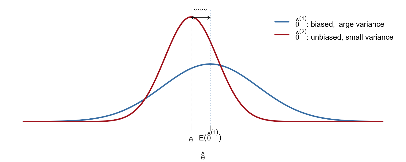
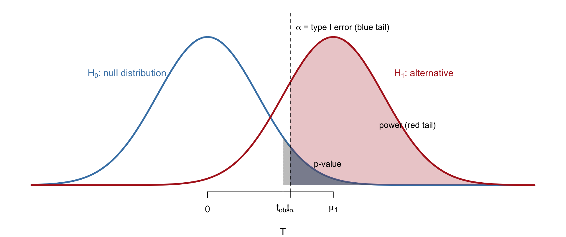
Figure 1.2: Shows how the error rates and the \(p\)-value of a hypothesis test all arise from the null and alternative distributions of a single test statistic. Null (\(H_0\)) and alternative (\(H_1\)) distributions of a test statistic \(T\), with the type I error, power, and \(p\)-value shown as tail areas.

Every quantity used to judge a hypothesis test is a tail probability computed from one of these two curves:

Quantity	Definition	Distribution used
\(p\)-value	\(P_{H_0}(T \ge t_{\text{obs}})\): probability, under \(H_0\), of a statistic at least as extreme as observed	null
Type I error \(\alpha\)	\(P_{H_0}(T \ge t_\alpha)\): probability of rejecting \(H_0\) when it is true	null
Power	\(P_{H_1}(T \ge t_\alpha)\): probability of correctly rejecting \(H_0\) when \(H_1\) holds	alternative

Computing any of these three numbers requires the same thing: the ability to evaluate a tail area of a distribution that, outside of the normal-theory special cases, is not available in closed form. Simulating the null and alternative distributions by repeated sampling — the same Monte Carlo idea used to study sampling distributions above — is often the most direct route when an exact formula does not exist.

1.1.7 Bayesian Inference

The Bayesian approach treats \(\theta\) itself as random, assigns it a prior distribution \(\pi(\theta)\) encoding what is known before the data arrive, and updates that belief with the likelihood via Bayes’ theorem to obtain the posterior, \[ p(\theta \mid x) = \frac{f(x \mid \theta)\,\pi(\theta)}{\int f(x \mid \theta)\,\pi(\theta)\, d\theta}. \] The numerator is easy: it is just the likelihood times the prior, both of which are specified. The denominator — the marginal likelihood or normalizing constant — is an integral over the entire parameter space, and for anything beyond a handful of conjugate textbook models, that integral has no closed form, especially once \(\theta\) has more than one or two components.

1.1.8 Prior, Likelihood, and Posterior

par(mar = c(4, 1, 1, 1))
# normal mean with known sigma: vague prior N(0, 3^2), n = 5, xbar = 2, sigma = 2
s2p <- 9; xbar <- 2; n <- 5; s2 <- 4
v_post <- 1 / (1 / s2p + n / s2); m_post <- v_post * (n * xbar / s2)
curve(dnorm(x, 0, sqrt(s2p)), -8, 8, lwd = 3, col = "gray40", lty = 2,
      axes = FALSE, xlab = expression(theta), ylab = "", ylim = c(0, 0.5))
curve(dnorm(x, xbar, sqrt(s2 / n)), add = TRUE, lwd = 3, col = "firebrick")
curve(dnorm(x, m_post, sqrt(v_post)), add = TRUE, lwd = 3, col = "steelblue")
axis(1)
legend("topleft", bty = "n", lwd = 3, lty = c(2, 1, 1),
       col = c("gray40", "firebrick", "steelblue"),
       legend = c(expression("vague prior "*pi(theta)),
                  expression("likelihood "*f(x*"|"*theta)),
                  expression("posterior "*p(theta*"|"*x))))

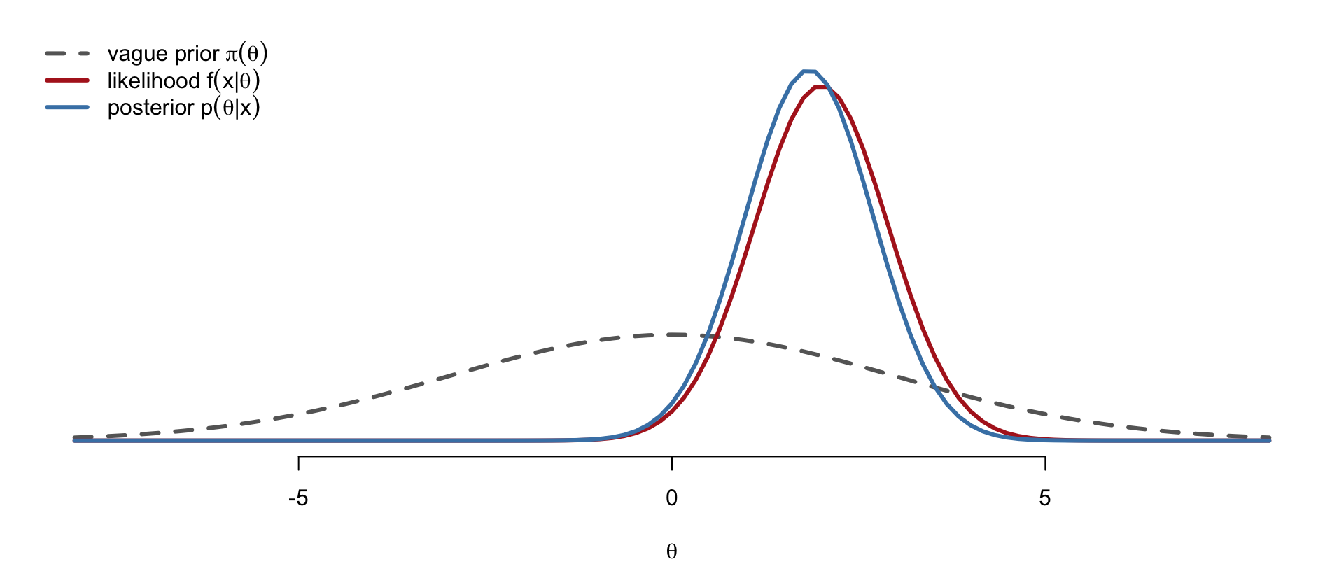
Figure 1.3: Previews Bayesian updating, in which the posterior combines the prior with the likelihood, here in a case where the data dominate the prior. A vague prior, the likelihood, and the resulting posterior for a normal mean: the posterior sits close to the likelihood, slightly narrower and pulled a little toward the prior mean.

In this normal-mean example the posterior can be written down exactly, and the picture makes the mechanism visible: a vague (wide, nearly flat) prior lets the likelihood dominate, so the posterior sits close to the likelihood, just slightly narrower and pulled a little toward the prior mean. Once the answer is available, inference reports posterior summaries — the posterior mean \(E(\theta \mid x)\), the posterior variance \(V(\theta \mid x)\), a credible interval, or a posterior probability \(P(\theta \in H_0 \mid x)\) — and every one of these summaries is, again, an integral against \(p(\theta \mid x)\). When the posterior itself has no closed form, none of its summaries do either.

1.1.9 Summary of the Three Tasks

Task	Object needed	Typical difficulty
Point estimation	Sampling distribution of \(\hat\theta\); maximizer of \(\ell(\theta)\)	No closed form
Hypothesis testing	Null distribution of \(T\)	Unknown for general data
Bayesian inference	\(\int f(x\mid\theta)\pi(\theta)\,d\theta\); \(E(\theta \mid x)\)	High-dimensional integral

Read across the rows, and a pattern emerges: each of the three classical tasks of statistical inference reduces to a computational problem — calculating a quantity accurately, simulating from a distribution that cannot be sampled directly, optimizing a function with no algebraic maximizer, or integrating over a parameter space with no closed-form antiderivative. None of these problems is solved by more statistical theory alone; all four are solved by numerical methods, which is what the rest of this course builds.

1.2 The Use of Computers in Statistics

The four computational tasks identified above — calculating, simulating, optimizing, integrating — organize the whole course. This section previews each one with a small example, and points ahead to the unit where it is developed properly.

1.2.1 1. Manipulating Numbers

Even simple calculations are not as trivial on a computer as they look on paper:

• \(1.1 + 2.1 + \cdots + 100.1\)
• \(S^2 = \sum_{i=1}^n (x_i - \bar x)^2 / (n-1)\)
• \(\prod_{i=1}^n f(x_i \mid \theta)\) for large \(n\)

A computer stores numbers with finite precision, so arithmetic that is exact on paper can go wrong in three specific ways: overflow, when a result is too large to represent and becomes Inf; underflow, when a result is too small and is rounded to zero; and rounding error, the gradual loss of significant digits as many operations accumulate. All three are silent — R will not raise an error — so a computation can return a plausible-looking but wrong number without any warning.

x <- c(1e10 + 1, 1e10 + 2, 1e10 + 3)
var(x)                                    # correct answer: 1

[1] 1

sum(x^2)/2 - 3 * mean(x)^2 / 2           # textbook formula

[1] 0

The two lines above compute the same variance by two algebraically equivalent formulas; they disagree because the second formula first squares numbers near \(10^{10}\) and then subtracts two similarly huge quantities, destroying most of the precision in the answer — a textbook illustration of catastrophic cancellation.

prod(dnorm(rnorm(1000)))                  # likelihood underflows to 0

[1] 0

sum(dnorm(rnorm(1000), log = TRUE))       # log-likelihood is fine

[1] -1459.311

Multiplying a thousand densities together underflows to exactly zero, even though the true likelihood is a small but perfectly well-defined positive number; summing the log-densities instead avoids the problem entirely, which is exactly why \(\ell(\theta) = \sum_i \log f(x_i \mid \theta)\), and not \(L(\theta) = \prod_i f(x_i \mid \theta)\), is the quantity every optimizer in this course actually works with. The unit on computer arithmetic develops these failure modes systematically — how floating-point numbers are stored, when each failure occurs, and the standard tricks (working on the log scale, the log-sum-exp identity, centering and scaling) that avoid them.

1.2.2 2. Simulation with Random Numbers

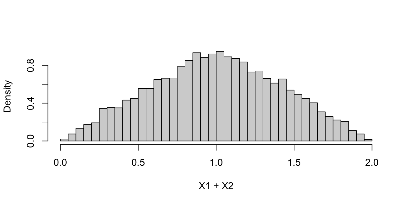
Monte Carlo methods replace a probability calculation that has no closed form with a large number of repeated random experiments, summarized numerically. The simplest possible illustration: if \(X_1, X_2\) are independent \(\text{Unif}(0,1)\) random variables, what is the distribution of \(X_1 + X_2\)? It can be worked out by hand (it is triangular on \([0, 2]\)), but it can also just be seen, by generating many pairs and plotting a histogram of their sums.

z <- runif(10000) + runif(10000)
hist(z, breaks = 40, freq = FALSE, main = "", xlab = "X1 + X2")

Figure 1.4: Demonstrates Monte Carlo simulation as a way of approximating a distribution, using an example whose exact answer is known so that the approximation can be checked. Simulated distribution of \(X_1 + X_2\) for independent \(\text{Unif}(0,1)\) variables, from 10,000 draws: a Monte Carlo approximation to the (triangular) true density.

The same idea scales up directly to the sampling-distribution question from earlier in this chapter. Repeating “draw \(x_1, \ldots, x_n\) from the assumed model, then compute the statistic” many times over gives an empirical approximation to the sampling distribution of any estimator or test statistic — \(\hat\mu^{(1)}\) versus \(\hat\mu^{(2)}\), the null distribution of \(T\) for non-normal data, the actual coverage of a nominal 95% confidence interval — without ever deriving a formula for it. The unit on random numbers and Monte Carlo develops this systematically: how pseudo-random numbers are generated, how draws from one distribution are transformed into draws from another, the Law of Large Numbers and Central Limit Theorem that justify treating a simulation average as an estimate, and how to use simulation to evaluate estimators and tests.

1.2.3 3. Optimization

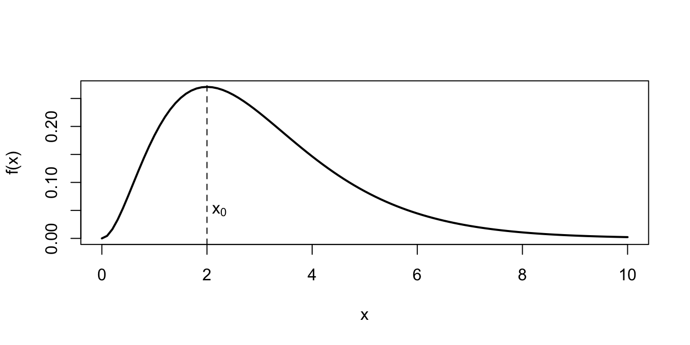
The MLE problem above is one instance of a completely general task: find \(x_0 = \arg\max_x f(x)\).

curve(dgamma(x, 3, 1), 0, 10, ylab = "f(x)", lwd = 2, main = "")
abline(v = 2, lty = 2)
text(2.1, 0.05, expression(x[0]), adj = 0)

Figure 1.5: A one-dimensional warm-up for numerical optimization, showing what it means to maximize a function before moving to problems that cannot be plotted. A Gamma(3,1) density: its maximizer \(x_0\) is obvious by eye, unlike a multi-parameter log-likelihood.

For a gamma density plotted over its whole domain, as above, the maximizer is obvious by eye. For a log-likelihood \(\ell(\theta)\) with many parameters, plotting is impossible and “obvious by eye” is not an option: the maximum has to be found by an iterative numerical search that starts somewhere and moves uphill. The unit on MLE and optimization develops these searches in order of increasing generality — bisection and golden-section search in one dimension, Newton–Raphson and Fisher scoring using derivative information, and gradient-based methods (BFGS, stochastic gradient descent) for high-dimensional problems where forming a Hessian is too expensive.

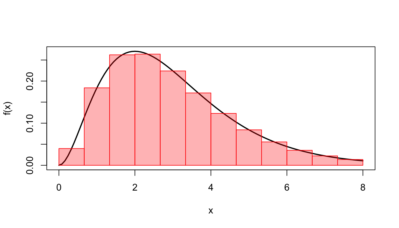
1.2.4 4. Advanced Simulation and Integration

The quantities that summarize a distribution are integrals: \[ E(X) = \int x f(x)\,dx, \qquad V(X), \qquad \int f(x\mid\theta)\pi(\theta)\,d\theta. \] Two broad strategies approximate an integral that has no closed form. Numerical quadrature approximates the area under the integrand by a sum of rectangles, trapezoids, or higher-order pieces; it is accurate and efficient in one or two dimensions, but its cost grows exponentially with the number of dimensions, which makes it impractical beyond a handful of parameters. Monte Carlo integration instead draws random points from (or related to) \(f\) and averages, trading the deterministic accuracy of quadrature for a convergence rate that does not depend on dimension — the only practical route once \(\theta\) has more than a few components. For a Bayesian posterior \(p(\theta \mid x)\), direct sampling is typically impossible because the normalizing constant is unknown, which is precisely the setting where Markov chain Monte Carlo (MCMC) is used: a Markov chain is constructed whose stationary distribution is the posterior itself, so that simulating the chain for long enough produces (dependent) draws from \(p(\theta \mid x)\) without ever having to evaluate the integral in its denominator.

f <- function(x) dgamma(x, 3, 1)
curve(f, 0, 8, lwd = 2, ylab = "f(x)", main = "")
k <- 12; xs <- seq(0, 8, length.out = k + 1)
rect(xs[-(k+1)], 0, xs[-1], f((xs[-(k+1)] + xs[-1]) / 2),
     col = adjustcolor("red", 0.3), border = "red")

Figure 1.6: Introduces numerical quadrature, the deterministic alternative to Monte Carlo for computing integrals, by turning the area under a density into a sum of rectangle areas. Numerical quadrature by rectangle rule: approximating the area under a Gamma(3,1) density with 12 midpoint rectangles.

The rectangles above illustrate the quadrature idea directly: \[ \int_a^b f(x)\,dx \approx \sum_{j=1}^k f(m_j)\,\Delta x, \] where \(m_j\) is the midpoint of the \(j\)th rectangle of width \(\Delta x\). The later units on numerical quadrature, Laplace approximation, rejection and importance sampling, and Markov chain Monte Carlo develop this strategy and its Monte Carlo counterpart from the ground up, culminating in the algorithms that make modern Bayesian computation possible.

1.2.5 Course Roadmap

Topic	Statistical task
Computer arithmetic	Reliable calculation of likelihoods and variances
Random numbers and Monte Carlo	Sampling distributions, evaluating estimators and tests
MLE and optimization	Point estimation without closed forms
Numerical integration and MCMC	Bayesian inference

Throughout the course, three themes recur alongside the statistical content: programming in R, writing vectorized code instead of explicit loops, and paying attention to the efficiency and numerical stability of the code itself — since, as the arithmetic examples above already show, a correct formula implemented carelessly can still give a wrong answer.