The last three chapters found a single best-fitting parameter value — the MLE — by optimization: gradient methods and Newton’s method for a smooth log-likelihood, EM when part of the data is missing. Bayesian inference asks a different question: not just where is the best \(\theta\), but how uncertain are we about it, given whatever we already believed before seeing the data? The answer is a full distribution over \(\theta\), not a point, and extracting anything useful from that distribution — a mean, a probability, a prediction — is almost always a matter of computing an integral or an optimization. That is why Bayesian inference sets the agenda for the rest of this book: numerical quadrature, Laplace’s method, rejection sampling, importance sampling, and Markov chain Monte Carlo are all, at bottom, different strategies for computing with a posterior distribution that has no closed form.
7.1 The Bayesian Framework
Bayesian inference treats the unknown parameter \(\theta\) itself as a random variable and proceeds in four steps:
Specify a prior\(\pi(\theta)\) — what is known or believed about \(\theta\) before seeing any data.
Specify a probability model for the data, \(P(y_1,\ldots,y_n\mid\theta)\), exactly the sampling model used to build a likelihood in the MLE chapters.
Find the posterior by Bayes’ rule, \[
P(\theta\mid y_{1:n}) = \frac{P(y_{1:n}\mid\theta)\,\pi(\theta)}
{\displaystyle\int P(y_{1:n}\mid\theta)\,\pi(\theta)\,d\theta}.
\]
Interpret the posterior: summarize \(\theta\), make predictions.
Writing \(L(\theta) = P(y_{1:n}\mid\theta)\) for the likelihood and \(f(\theta) = L(\theta)\pi(\theta)\) for the unnormalized posterior — the notation used throughout the rest of this book — step 3 becomes \[
P(\theta\mid y_{1:n}) = \frac{f(\theta)}{P(y_{1:n})}, \qquad
P(y_{1:n}) = \int f(\theta)\,d\theta.
\]\(P(y_{1:n})\), the marginal likelihood, is the likelihood averaged over the prior rather than maximized over \(\theta\); it does not depend on \(\theta\), so it plays no role in shaping the posterior, but it is usually the hardest single quantity in the whole framework to compute — it is a \(p\)-dimensional integral with no generic closed form, and it is the running example of the next three chapters (numerical quadrature, Laplace approximation, and the Monte Carlo methods after that).
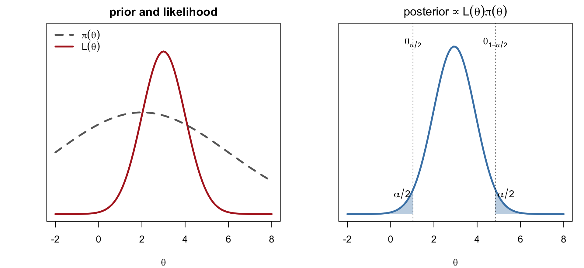
Figure 7.1: Shows how Bayes’ rule combines a prior with a likelihood into a posterior, and how a credible interval is read off from the posterior. Left: a flat-ish prior \(\pi(\theta)\) (dashed) and a likelihood \(L(\theta)\) (solid) that is much more concentrated — the data are far more informative than the prior here. Right: the posterior \(\propto L(\theta)\pi(\theta)\), essentially the (renormalized) likelihood since the prior is so flat over the region where \(L\) has mass. Shaded tails cut off \(\alpha/2\) of the posterior probability each, giving a \((1-\alpha)\) credible interval \((\theta_{\alpha/2},\theta_{1-\alpha/2})\).
7.2 Summarizing the Posterior
7.2.1 Point estimates from loss functions
A single number for \(\theta\) is a decision, and a principled way to make a decision is to minimize expected loss. Given a loss function \(L(\theta,\hat\theta)\) measuring the cost of reporting \(\hat\theta\) when the truth is \(\theta\), the Bayes estimate minimizes the posterior expected loss, \[
\hat\theta = \arg\min_{\hat\theta}\; E\big[L(\theta,\hat\theta)\mid y_{1:n}\big]
= \arg\min_{\hat\theta} \int L(\theta,\hat\theta)\,P(\theta\mid y_{1:n})\,d\theta.
\] Three standard losses give three familiar summaries:
Interval estimates go one step further: a \((1-\alpha)\)credible interval\((\theta_{\alpha/2},\theta_{1-\alpha/2})\) contains \(\theta\) with posterior probability \(1-\alpha\) — a direct probability statement about \(\theta\) itself, unlike a frequentist confidence interval, whose \(1-\alpha\) coverage is a statement about the procedure across repeated samples, not about \(\theta\) given the data actually observed.
Every entry in that table is either an integral (a mean, a median, a probability) or an optimization (the mode) over the posterior. This is the sense in which Bayesian inference is inherently computational: even the most basic summaries require operations that, outside of conjugate models like the three worked below, have no closed form.
7.2.2 Posterior prediction
Often the real target is not \(\theta\) itself but a future observation. The posterior predictive distribution of \(y_{n+1}\) is \[
P(y_{n+1}\mid y_{1:n}) = \frac{\int P(y_{n+1},y_{1:n}\mid\theta)\,\pi(\theta)\,d\theta}
{\int P(y_{1:n}\mid\theta)\,\pi(\theta)\,d\theta}.
\] If \(y_1,\ldots,y_n,y_{n+1}\) are conditionally independent given \(\theta\) — the usual iid-sampling assumption — the joint density factors and this simplifies to \[
P(y_{n+1}\mid y_{1:n}) = \int P(y_{n+1}\mid\theta)\,P(\theta\mid y_{1:n})\,d\theta,
\] an average of the sampling density over the posterior, rather than the sampling density evaluated at one plug-in estimate \(\hat\theta\). Given posterior draws \(\theta_1,\ldots,\theta_J\sim P(\theta\mid y_{1:n})\) (the subject of the Monte Carlo chapters later in the book), \[
P(y_{n+1}\mid y_{1:n}) \approx \frac1J\sum_{j=1}^J P(y_{n+1}\mid\theta_j).
\] Because it mixes over the whole posterior instead of conditioning on a single \(\hat\theta\), the predictive distribution is necessarily wider than any individual \(P(y_{n+1}\mid\theta_j)\): it carries both the sampling variability and the remaining uncertainty about \(\theta\). The Poisson–Gamma example below makes this concrete with a closed-form predictive distribution that is visibly overdispersed relative to a plug-in Poisson.
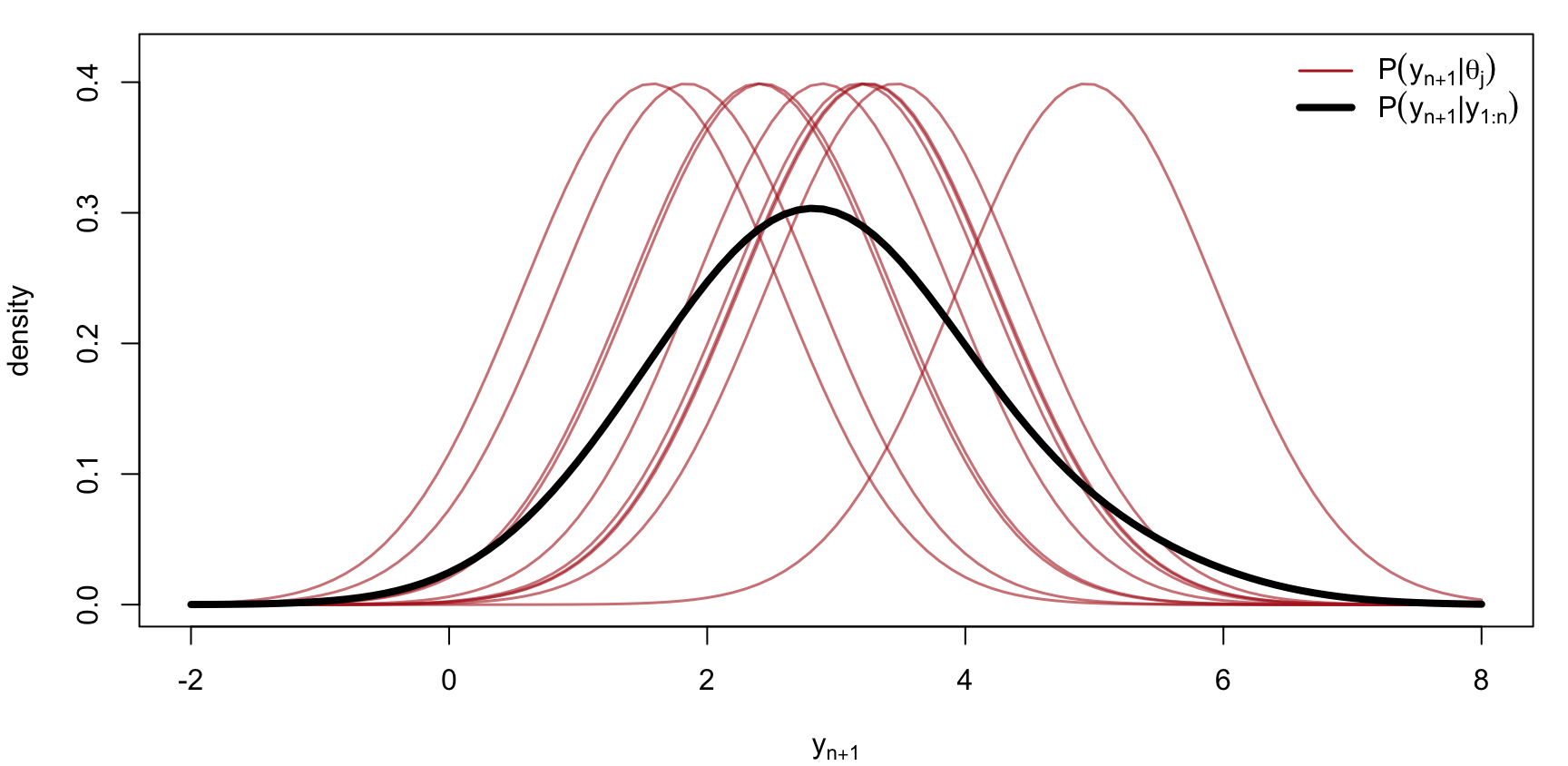
Figure 7.2: Shows how the posterior predictive distribution is built by averaging the sampling density over the posterior, so that it accounts for uncertainty about the parameter. Red: the sampling density \(P(y_{n+1}\mid\theta_j)\) for ten posterior draws \(\theta_j\sim N(3, 0.8^2)\). Black: their average, the posterior predictive density \(P(y_{n+1}\mid y_{1:n})\). The predictive is visibly wider than any single red curve — it inherits both the spread of \(P(y_{n+1}\mid\theta)\) and the spread of the \(\theta_j\).
7.3 Example: Bernoulli Data with a Beta Prior
7.3.1 Prior
Let \(y_1,\ldots,y_n\mid\theta \overset{iid}{\sim}\text{Bern}(\theta)\), with \(\theta\in(0,1)\) a success probability, and give \(\theta\) a \(\text{Beta}(\alpha_1,\alpha_0)\) prior, \(\alpha_1,\alpha_0>0\) given: \[
\pi(\theta) = \frac{\Gamma(\alpha_0+\alpha_1)}{\Gamma(\alpha_0)\Gamma(\alpha_1)}\,
\theta^{\alpha_1-1}(1-\theta)^{\alpha_0-1}, \qquad 0<\theta<1,
\]\[
E(\theta) = \frac{\alpha_1}{\alpha_0+\alpha_1}, \qquad
V(\theta) = \frac{\alpha_0\alpha_1}{(\alpha_0+\alpha_1)^2(\alpha_0+\alpha_1+1)}.
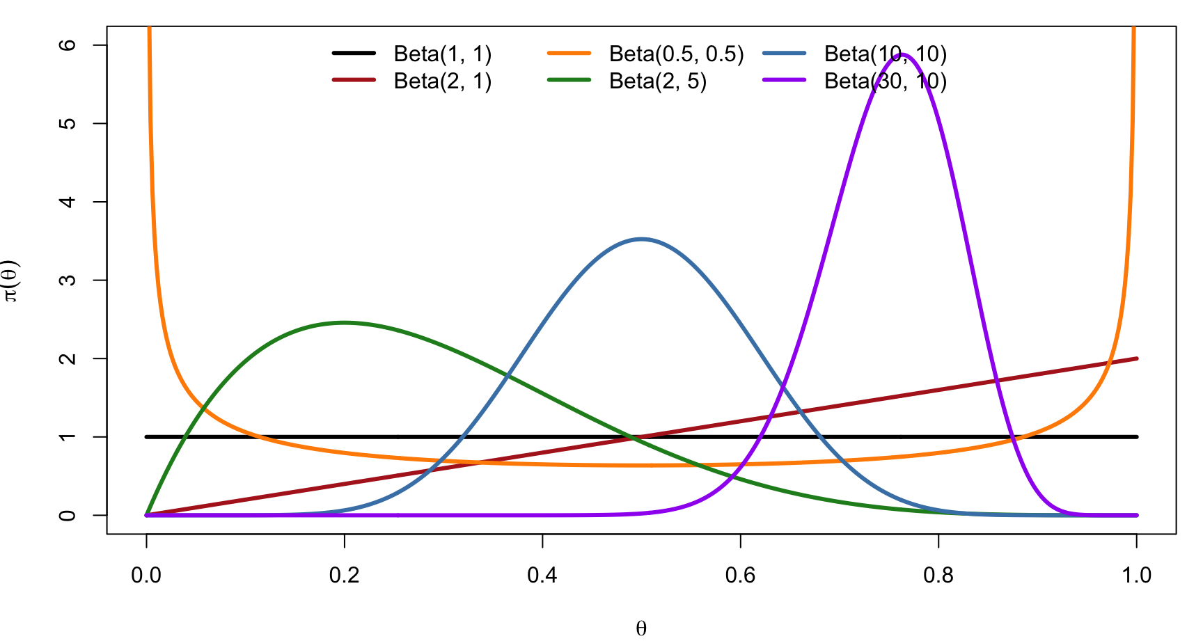
\] The parameters have a direct reading as pseudo-data: \(\alpha_1\) behaves like a prior count of successes, \(\alpha_0\) a prior count of failures, and \(\alpha_0+\alpha_1\) a prior “sample size” — the more of it, the more concentrated \(\pi(\theta)\) is around \(\alpha_1/(\alpha_0+\alpha_1)\), exactly as a real sample of that size would concentrate a Bernoulli proportion. \(\text{Beta}(1,1)\) is \(\text{Unif}(0,1)\), a genuinely flat prior; small \(\alpha\)’s (e.g. \(\text{Beta}(0.5,0.5)\)) give a U-shaped prior that expects \(\theta\) near \(0\) or \(1\); large, unequal \(\alpha\)’s concentrate the prior away from \(\tfrac12\).
Figure 7.3: Shows the range of prior beliefs about a probability that the Beta family can express, to guide the choice of a prior. Six Beta priors spanning flat, U-shaped, and concentrated shapes. Beta(1,1) is uniform; Beta(0.5,0.5) is U-shaped, favouring \(\theta\) near the boundaries; Beta(2,5) and Beta(30,10) are increasingly concentrated, at \(\theta\approx2/7\) and \(\theta\approx0.75\) respectively.
7.3.2 Likelihood and posterior
With \(P(y_i\mid\theta) = \theta^{y_i}(1-\theta)^{1-y_i}\) and \(\mathbf y = (y_1,\ldots,y_n)\), the likelihood depends on the data only through the total number of successes: \[
L(\theta) = \prod_{i=1}^n \theta^{y_i}(1-\theta)^{1-y_i} = \theta^{n_1}(1-\theta)^{n_0},
\qquad n_1 = \sum_i y_i,\ \ n_0 = n - n_1.
\] Multiplying by the prior and collecting powers of \(\theta\) and \(1-\theta\), \[
f(\theta) = \pi(\theta)L(\theta) \;\propto\; \theta^{\alpha_1-1}(1-\theta)^{\alpha_0-1}\cdot\theta^{n_1}(1-\theta)^{n_0}
= \theta^{(\alpha_1+n_1)-1}(1-\theta)^{(\alpha_0+n_0)-1}.
\] This unnormalized posterior is, up to the constant \(P(\mathbf y)\), exactly the Beta kernel with updated parameters \(\alpha_1' = \alpha_1+n_1\), \(\alpha_0' = \alpha_0+n_0\) — and since a Beta density is the only normalized distribution with that kernel, \[
\theta\mid\mathbf y \sim \text{Beta}(\alpha_1+n_1,\ \alpha_0+n_0)
\] follows immediately, with no integration needed. This is what it means for the Beta prior to be conjugate to the Bernoulli likelihood: updating the prior to the posterior is nothing but arithmetic on the two parameters, \(\alpha_1 \to \alpha_1+n_1\), \(\alpha_0\to\alpha_0+n_0\), and the marginal likelihood \(P(\mathbf y)\) never has to be computed explicitly, because matching the two Beta kernels pins down the normalizing constant for free. Few models have this property; it is a stroke of algebraic luck rather than a general feature of Bayesian inference, which is exactly why the rest of this book is needed.
7.3.3 Posterior summaries
The pseudo-data reading of \(\alpha_1,\alpha_0\) carries through to the posterior mean, which is an exact weighted average of the prior mean and the MLE \(\hat\theta_{\text{MLE}} = n_1/n\): \[
E(\theta\mid\mathbf y) = \frac{\alpha_1+n_1}{\alpha_0+\alpha_1+n}
= \underbrace{\frac{\alpha_0+\alpha_1}{\alpha_0+\alpha_1+n}}_{w}\cdot\frac{\alpha_1}{\alpha_0+\alpha_1}
+ (1-w)\cdot\hat\theta_{\text{MLE}}.
\] The weight \(w\) on the prior mean is the prior’s pseudo-sample-size relative to the total (prior plus real) sample size; as \(n\to\infty\), \(w\to0\) and the posterior mean converges to the MLE regardless of the prior. The posterior variance, \[
V(\theta\mid\mathbf y) = \frac{(\alpha_1+n_1)(\alpha_0+n_0)}{(n+\alpha_0+\alpha_1)^2(n+\alpha_0+\alpha_1+1)} = O\!\left(\frac1n\right),
\] shrinks at the same \(1/n\) rate as the sampling variance of the MLE, \(\hat\theta_{\text{MLE}}\,\dot\sim\,N\big(\theta_0,\,1/(nI(\theta_0))\big)\) from the MLE chapters — for large \(n\) the two approaches to uncertainty agree, with the prior’s influence vanishing.
7.3.4 The marginal likelihood in closed form
Because conjugacy gives the whole posterior in closed form, it also gives the marginal likelihood \(P(\mathbf y)=\int_0^1 f(\theta)\,d\theta\) in closed form, by integrating the unnormalized Beta kernel directly against its own normalizing constant: \[
P(\mathbf y) = \frac{\Gamma(\alpha_0+\alpha_1)}{\Gamma(\alpha_0)\Gamma(\alpha_1)}
\int_0^1 \theta^{(\alpha_1+n_1)-1}(1-\theta)^{(\alpha_0+n_0)-1}\,d\theta
= \frac{\Gamma(\alpha_0+\alpha_1)}{\Gamma(\alpha_0)\Gamma(\alpha_1)}\cdot
\frac{\Gamma(\alpha_1+n_1)\,\Gamma(\alpha_0+n_0)}{\Gamma(\alpha_0+\alpha_1+n)},
\] using \(\int_0^1\theta^{a-1}(1-\theta)^{b-1}\,d\theta = B(a,b) =
\Gamma(a)\Gamma(b)/\Gamma(a+b)\). On the log scale, with \(\log B(a,b)=\log\Gamma(a)+\log\Gamma(b)-\log\Gamma(a+b)\), \[
\log P(\mathbf y) = \log B(\alpha_1+n_1,\ \alpha_0+n_0) - \log B(\alpha_1,\ \alpha_0).
\] This exact Beta–Bernoulli conjugate identity is the same trick used for Gamma–Poisson and Normal–Normal below: matching a recognizable kernel against its own normalizing constant hands over \(P(\mathbf y)\) for free, with no numerical integration anywhere.
7.3.5 Posterior predictive, in closed form
For a new \(y_{n+1}\mid\theta\sim\text{Bern}(\theta)\), the general predictive formula from earlier in this chapter simplifies beautifully in the conjugate case, because \(E(\theta\mid\mathbf y)\)is the predictive success probability: \[
P(y_{n+1}=1\mid\mathbf y) = \int_0^1 \theta\, P(\theta\mid\mathbf y)\,d\theta = E(\theta\mid\mathbf y),
\qquad y_{n+1}\mid\mathbf y \sim \text{Bern}\big(E(\theta\mid\mathbf y)\big).
\] This exact equality (\(E(\theta\mid\mathbf y)\) doing double duty as both a point estimate of \(\theta\) and the predictive probability of success) is special to Bernoulli data; the Poisson–Gamma and Normal–Normal examples below give predictive distributions that are genuinely wider than their plug-in sampling models.
7.3.6 Worked numbers: the complete inference output
Take a near-flat \(\text{Beta}(1,1)\) prior and \(n=10\) trials with \(y=7\) successes. The table below collects everything derived above — marginal likelihood, posterior, its mean/sd and credible interval, and the predictive distribution — in one place, and the same five quantities are computed the same way for the Gamma–Poisson and Normal–Normal examples that follow:
Table 7.1: Collects every quantity reported in a conjugate Beta-Binomial analysis, from the prior and MLE to the posterior, credible interval, and predictive distribution. Complete inference output, Beta(1,1) prior with n = 10, y = 7.
quantity
value
prior mean
0.500
MLE (\(y/n\))
0.700
log marginal likelihood
-7.185
posterior distribution
Beta(8, 4)
posterior mean
0.667
posterior sd
0.131
95% credible interval
(0.390, 0.891)
predictive distribution
Bernoulli(0.667)
predictive mean
0.667
predictive sd
0.471
With a uniform prior the posterior mean \(0.667\) sits between the prior mean \(0.5\) and the MLE \(0.7\), pulled almost all the way to the MLE because the prior carries only \(\alpha_0+\alpha_1=2\) pseudo-observations against \(10\) real ones. The 95% credible interval, \((0.390, 0.891)\), is read directly off the Beta CDF (qbeta) — no simulation, no quadrature, because conjugacy already handed over the exact posterior family. The predictive distribution \(\text{Bern}(0.667)\) has the same mean as the posterior but a nonzero sd (\(0.471\)), because even a Bernoulli outcome is uncertain even once \(\theta\) is known exactly.
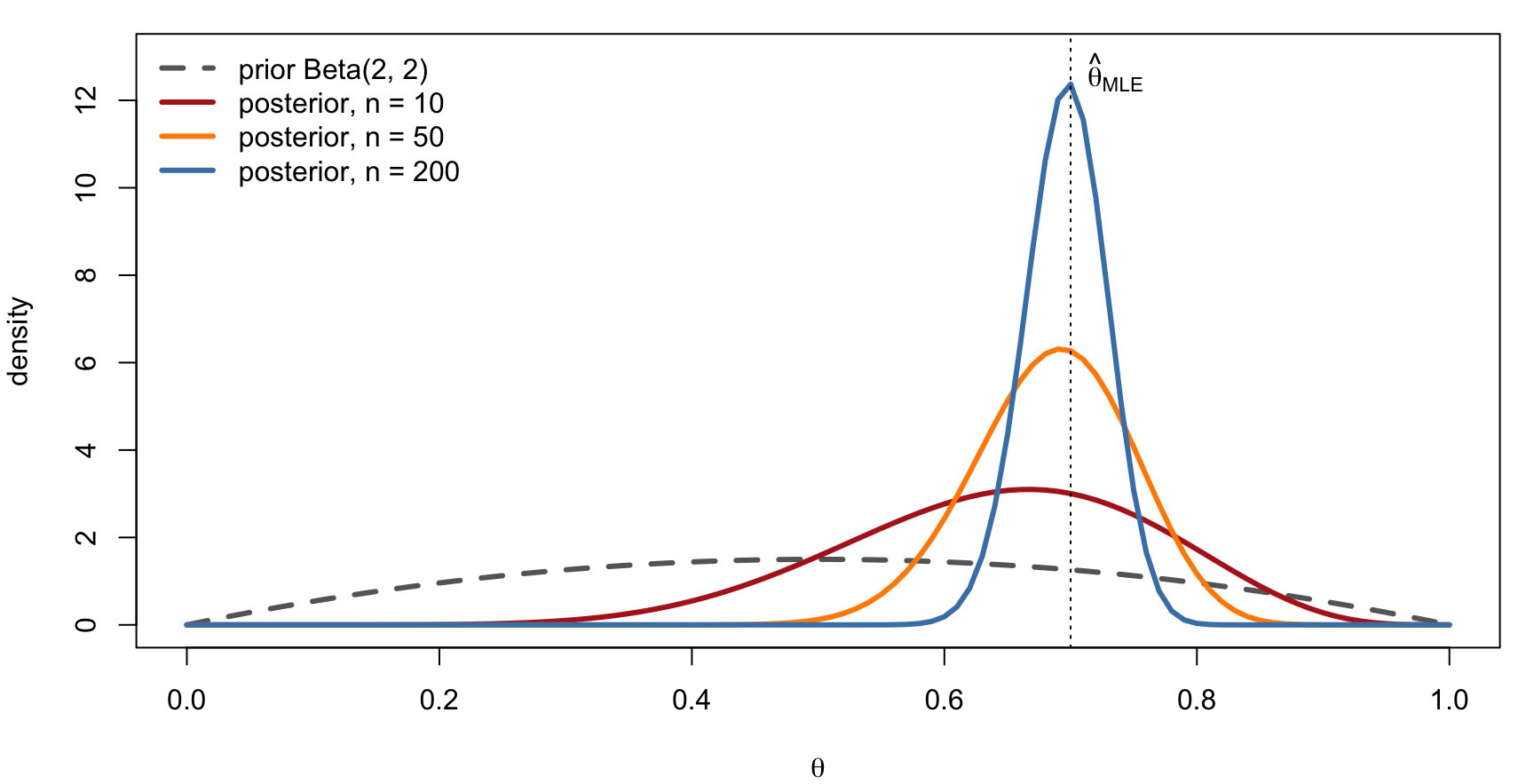
Figure 7.4: Shows how the influence of the prior fades as data accumulate, so that the posterior concentrates around the MLE. Prior Beta(2,2) (dashed) and posteriors after \(n=10,50,200\) observations with \(\bar y=0.7\) held fixed. The posterior narrows at rate \(1/\sqrt n\) and moves onto the MLE as \(n\) grows, exactly the \(w\to0\) argument above made visible.
7.4 Example: Poisson Data with a Gamma Prior
7.4.1 Prior
Now let \(y_1,\ldots,y_n\mid\lambda \overset{iid}{\sim}\text{Poisson}(\lambda)\), \(\lambda>0\) a rate, with a \(\text{Gamma}(\alpha,\beta)\) prior (shape \(\alpha\), rate \(\beta\)), \[
\pi(\lambda) = \frac{\beta^\alpha}{\Gamma(\alpha)}\lambda^{\alpha-1}e^{-\beta\lambda}, \qquad \lambda>0,
\qquad E(\lambda) = \frac{\alpha}{\beta}, \qquad V(\lambda) = \frac{\alpha}{\beta^2}.
\] The pseudo-data reading again applies, with the two parameters playing different roles than in the Beta case: \(\alpha\) behaves like a prior total count and \(\beta\) like a prior total exposure (a number of pseudo time-units or pseudo-observations already seen with rate \(\lambda\)), so \(\alpha/\beta\) is a prior average rate — the same “counts per exposure” structure as \(\hat\lambda_{\text{MLE}} = \sum y_i / n\), with \(\beta\) playing the role \(n\) plays in the likelihood.
7.4.2 Likelihood and posterior
With \(P(y_i\mid\lambda) = \lambda^{y_i}e^{-\lambda}/y_i!\), the likelihood depends on the data only through the total count \(S=\sum_i y_i\): \[
L(\lambda) = \prod_{i=1}^n \frac{\lambda^{y_i}e^{-\lambda}}{y_i!}
= \frac{\lambda^{S}e^{-n\lambda}}{\prod_i y_i!}, \qquad S = \sum_{i=1}^n y_i.
\] Multiplying by the prior and collecting powers of \(\lambda\) and \(e^{-\lambda}\), \[
f(\lambda) = \pi(\lambda)L(\lambda) \;\propto\; \lambda^{\alpha-1}e^{-\beta\lambda}\cdot\lambda^{S}e^{-n\lambda}
= \lambda^{(\alpha+S)-1}e^{-(\beta+n)\lambda},
\] the kernel of a \(\text{Gamma}(\alpha+S,\ \beta+n)\) density. The Gamma prior is therefore conjugate to the Poisson likelihood, exactly as Beta was to Bernoulli, and by the same argument (matching a recognizable kernel pins down the normalizing constant automatically): \[
\lambda\mid\mathbf y \sim \text{Gamma}(\alpha+S,\ \beta+n).
\] The posterior mean has precisely the weighted-average structure seen in the Bernoulli case, with \(\beta\) now playing the role \(\alpha_0+\alpha_1\) played there: \[
E(\lambda\mid\mathbf y) = \frac{\alpha+S}{\beta+n}
= \underbrace{\frac{\beta}{\beta+n}}_{w}\cdot\frac{\alpha}{\beta}
+ (1-w)\cdot\underbrace{\frac{S}{n}}_{\hat\lambda_{\text{MLE}}},
\] a weighted average of the prior mean and the MLE, with prior weight \(w=\beta/(\beta+n)\to0\) as \(n\to\infty\) — the same shrinkage story as Beta–Bernoulli, now driven by \(\beta\) (prior pseudo-exposure) instead of \(\alpha_0+\alpha_1\) (prior pseudo-sample-size).
7.4.3 The marginal likelihood in closed form
Because conjugacy gives the whole posterior in closed form, it also gives the marginal likelihood \(P(\mathbf y)=\int f(\lambda)\,d\lambda\) in closed form, by integrating the unnormalized Gamma kernel directly against its own normalizing constant: \[
P(\mathbf y) = \left(\prod_{i=1}^n \frac1{y_i!}\right)\frac{\beta^\alpha}{\Gamma(\alpha)}
\int_0^\infty \lambda^{(\alpha+S)-1}e^{-(\beta+n)\lambda}\,d\lambda
= \left(\prod_{i=1}^n \frac1{y_i!}\right)\frac{\beta^\alpha\,\Gamma(\alpha+S)}{\Gamma(\alpha)\,(\beta+n)^{\alpha+S}},
\] using \(\int_0^\infty \lambda^{k-1}e^{-c\lambda}\,d\lambda = \Gamma(k)/c^k\). On the log scale, \[
\log P(\mathbf y) = \alpha\log\beta - \log\Gamma(\alpha) + \log\Gamma(\alpha+S)
- (\alpha+S)\log(\beta+n) - \sum_{i=1}^n \log(y_i!).
\] This exact Gamma–Poisson conjugate identity is what makes the Poisson-rate model a useful test case for approximate methods: the Laplace approximation chapter later in this book applies its mode-and-curvature approximation to this same model and checks the result against precisely this formula, since here — unlike in most applications — the truth is known.
7.4.4 Posterior predictive, in closed form
For a new count \(y_{n+1}\mid\lambda\sim\text{Poisson}(\lambda)\), integrating the Poisson sampling density against the \(\text{Gamma}(\alpha+S,\beta+n)\) posterior gives a Negative Binomial predictive distribution, \[
P(y_{n+1}\mid\mathbf y) = \int_0^\infty \frac{\lambda^{y_{n+1}}e^{-\lambda}}{y_{n+1}!}\,
\frac{(\beta+n)^{\alpha+S}}{\Gamma(\alpha+S)}\lambda^{(\alpha+S)-1}e^{-(\beta+n)\lambda}\,d\lambda
= \text{NegBin}\!\left(\text{size}=\alpha+S,\ \ p=\frac{\beta+n}{\beta+n+1}\right),
\] by the same Gamma-integral identity used for the marginal likelihood above. Its mean matches the posterior mean of \(\lambda\) exactly (as it must, by the tower property), but its variance is larger than that of a plug-in Poisson at the posterior mean rate: \[
E(y_{n+1}\mid\mathbf y) = \frac{\alpha+S}{\beta+n}, \qquad
V(y_{n+1}\mid\mathbf y) = \frac{\alpha+S}{\beta+n}\left(1+\frac1{\beta+n}\right)
= E(y_{n+1}\mid\mathbf y)\cdot\Big(1+\tfrac{1}{\beta+n}\Big).
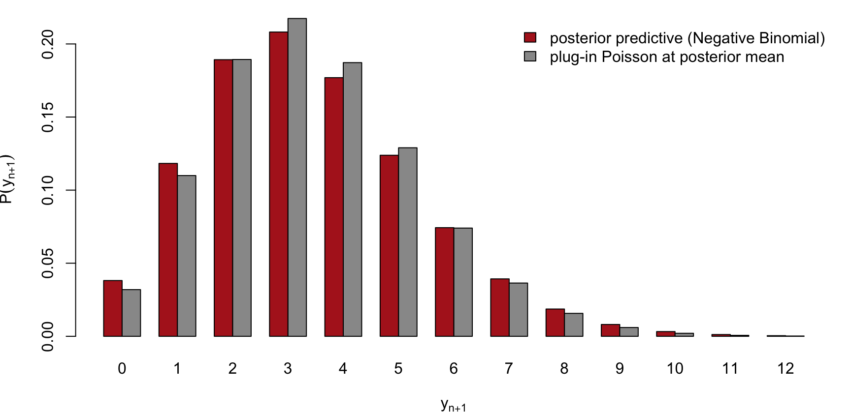
\] A plug-in Poisson at \(\lambda=E(\lambda\mid\mathbf y)\) would have variance equal to its mean — the extra factor \(1+1/(\beta+n)\) is entirely the posterior uncertainty about \(\lambda\) leaking into the prediction, exactly the “wider than any single \(P(y_{n+1}\mid\theta_j)\)” phenomenon from the general framework above, now with an explicit formula for how much wider.
7.4.5 Worked numbers: the complete inference output
Take \(\text{Gamma}(2,1)\) as the prior (prior mean \(2\), i.e. a mild belief that the rate is around \(2\), with pseudo-exposure \(\beta=1\)) and \(n=8\) simulated counts from a true rate of \(3\). The table collects the same five quantities as the Beta–Bernoulli table above — marginal likelihood, posterior, its mean/sd and credible interval, and the predictive distribution:
Table 7.2: Collects every quantity reported in a conjugate Poisson-Gamma analysis, from the prior and MLE to the posterior, credible interval, and predictive distribution. Complete inference output, Gamma(2,1) prior, n = 8 Poisson counts.
quantity
value
data \(y_{1:8}\)
5, 6, 2, 5, 3, 3, 4, 1
sum \(S\)
29
prior mean
2.000
MLE (\(S/n\))
3.625
log marginal likelihood
-17.065
posterior distribution
Gamma(31, 9)
posterior mean
3.444
posterior sd
0.619
95% credible interval
(2.340, 4.759)
predictive distribution
NegBin(31, 0.900)
predictive mean
3.444
predictive sd
1.956
The MLE, \(29/8=3.625\), and the prior mean, \(2\), are pulled toward each other by the posterior mean \(3.444\) — mostly toward the MLE, since the prior’s pseudo-exposure \(\beta=1\) is small next to the real \(n=8\). Compare this to the true generating rate of \(3\): both the MLE and the posterior mean overshoot it here (this particular simulated sample happened to run a bit high), and the 95% credible interval \((2.340, 4.759)\) still comfortably covers it. With \(\beta+n=9\), the predictive sd \(1.957\) exceeds the plug-in Poisson sd \(\sqrt{3.444}=1.856\) by the factor \(\sqrt{1+1/9}\) — the same overdispersion story made numeric.
7.4.6 Overdispersion, visualized
The gap is small here because \(n\) is already large relative to the prior, but it widens as \(n\) shrinks or the prior gets vaguer (smaller \(\beta\)). The figure below makes the same point on the density scale: the predictive has visibly heavier tails than a plug-in Poisson with the same mean.
Figure 7.5: Shows why the posterior predictive distribution is more dispersed than a plug-in prediction: it also reflects the remaining uncertainty about the Poisson rate. Posterior predictive \(P(y_{n+1}\mid\mathbf y)\) (Negative Binomial, red) against a plug-in Poisson at the posterior mean rate (gray). Same mean, but the predictive has heavier tails: the two bars noticeably diverge above \(y_{n+1}=7\), and \(V(y_{n+1}\mid\mathbf y)\) exceeds the plug-in variance by the factor \(1+1/(\beta+n)=1.111\) derived above.
7.5 Example: Normal Data with a Normal Prior (Known Variance)
7.5.1 Prior
Now let \(y_1,\ldots,y_n\mid\mu \overset{iid}{\sim} N(\mu,\sigma^2)\), with \(\sigma^2\)known/fixed and only the mean \(\mu\in\mathbb R\) unknown. Give \(\mu\) a Normal prior, parametrized through a prior pseudo-sample-size \(\kappa_0>0\) so that it lines up with the pseudo-data reading used in the two examples above: \[
\pi(\mu) = N\!\Big(\mu_0,\ \frac{\sigma^2}{\kappa_0}\Big), \qquad
E(\mu) = \mu_0, \qquad V(\mu) = \frac{\sigma^2}{\kappa_0}.
\]\(\mu_0\) is the prior guess for \(\mu\), and \(\kappa_0\) counts how many pseudo-observations (each with the known variance \(\sigma^2\)) that guess is worth: large \(\kappa_0\) means a confident, concentrated prior; \(\kappa_0\to0\) recovers a flat, uninformative prior on \(\mu\).
7.5.2 Likelihood and posterior
With \(P(y_i\mid\mu) = (2\pi\sigma^2)^{-1/2}\exp\{-(y_i-\mu)^2/(2\sigma^2)\}\), the likelihood depends on the data only through the sample mean \(\bar y = \frac1n\sum_i y_i\): \[
L(\mu) \;\propto\; \exp\left\{-\frac1{2\sigma^2}\sum_{i=1}^n(y_i-\mu)^2\right\}
\;\propto\; \exp\left\{-\frac{n(\mu-\bar y)^2}{2\sigma^2}\right\}.
\] Multiplying by the prior and completing the square in \(\mu\), \[
f(\mu) = \pi(\mu)L(\mu) \;\propto\;
\exp\left\{-\frac{(\mu-\mu_0)^2}{2\sigma^2/\kappa_0} - \frac{n(\mu-\bar y)^2}{2\sigma^2}\right\}
\;\propto\; \exp\left\{-\frac{(\mu-\mu_n)^2}{2\sigma^2/\kappa_n}\right\},
\] the kernel of a Normal density with \[
\kappa_n = \kappa_0+n, \qquad \mu_n = \frac{\kappa_0\mu_0+n\bar y}{\kappa_0+n}.
\] The Normal prior is therefore conjugate to the Normal likelihood (known variance), exactly as Beta was to Bernoulli and Gamma to Poisson: \[
\mu\mid\mathbf y \sim N\!\Big(\mu_n,\ \frac{\sigma^2}{\kappa_n}\Big).
\] As in the other two models, the posterior mean is a pseudo-sample-size weighted average of the prior mean and the MLE \(\hat\mu_{\text{MLE}}=\bar y\), \[
\mu_n = \underbrace{\frac{\kappa_0}{\kappa_0+n}}_{w}\cdot\mu_0 + (1-w)\cdot\bar y,
\] with prior weight \(w=\kappa_0/(\kappa_0+n)\to0\) as \(n\to\infty\), and the posterior “pseudo-sample-sizes” simply add: \(\kappa_n=\kappa_0+n\) — posterior precision (inverse variance, in units of \(1/\sigma^2\)) is prior precision plus data precision.
7.5.3 The marginal likelihood in closed form
Because conjugacy gives the whole posterior in closed form, it also gives the marginal likelihood \(P(\mathbf y)=\int f(\mu)\,d\mu\) in closed form. Writing the likelihood with its full normalizing constant, \(L(\mu)=(2\pi\sigma^2)^{-n/2}\exp\{-SS/(2\sigma^2)\}\exp\{-n(\mu-\bar y)^2/(2\sigma^2)\}\) with \(SS=\sum_{i=1}^n(y_i-\bar y)^2\), and integrating the same Gaussian-kernel product used to find the posterior above (a standard Gaussian-product identity: \(\int\exp\{-a(\mu-m_1)^2/2-b(\mu-m_2)^2/2\}\,d\mu
=\sqrt{2\pi/(a+b)}\exp\{-ab(m_1-m_2)^2/(2(a+b))\}\)) gives \[
P(\mathbf y) = (2\pi\sigma^2)^{-n/2}\sqrt{\frac{\kappa_0}{\kappa_n}}\,
\exp\left\{-\frac{SS}{2\sigma^2} - \frac{\kappa_0 n(\mu_0-\bar y)^2}{2\sigma^2\kappa_n}\right\}.
\] On the log scale, \[
\log P(\mathbf y) = -\frac n2\log(2\pi\sigma^2) + \frac12\log\frac{\kappa_0}{\kappa_n}
- \frac{SS}{2\sigma^2} - \frac{\kappa_0 n(\mu_0-\bar y)^2}{2\sigma^2\kappa_n}.
\] As in the other two models, matching the Normal kernel of \(f(\mu)\) against its own normalizing constant hands over \(P(\mathbf y)\) with no numerical integration.
7.5.4 Posterior predictive, in closed form
For a new \(y_{n+1}\mid\mu\sim N(\mu,\sigma^2)\), integrating the Normal sampling density against the \(N(\mu_n,\sigma^2/\kappa_n)\) posterior — a sum of independent Normals — gives another Normal predictive distribution, \[
y_{n+1}\mid\mathbf y \sim N\!\Big(\mu_n,\ \sigma^2\big(1+\tfrac1{\kappa_n}\big)\Big),
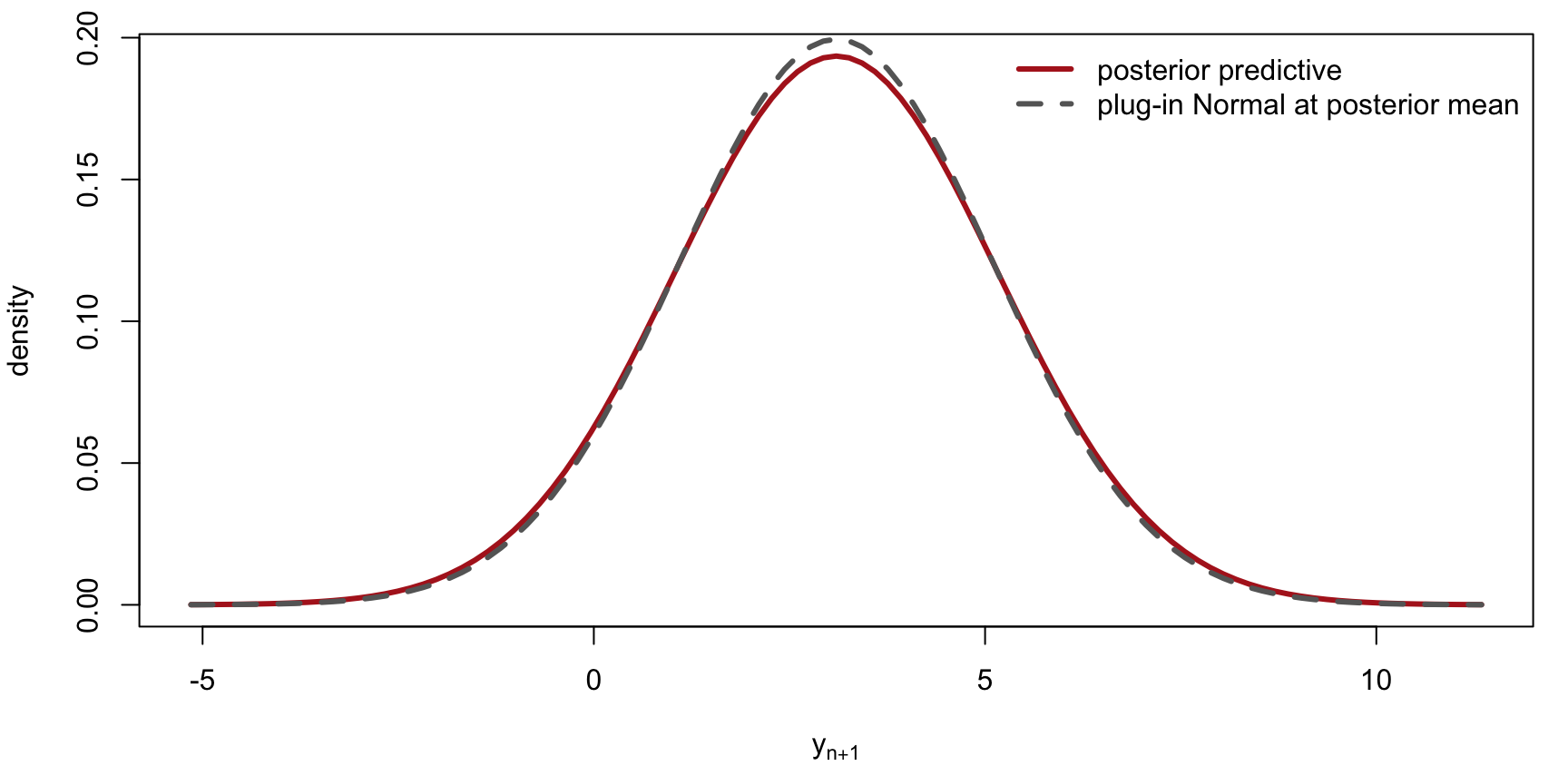
\] with mean equal to the posterior mean of \(\mu\) (as it must, by the tower property) and variance larger than the known sampling variance \(\sigma^2\) by exactly the factor \(1+1/\kappa_n\) — the same form as the Gamma–Poisson predictive-variance inflation above, now for a continuous outcome: the extra \(1/\kappa_n\) is the leftover posterior uncertainty about \(\mu\) leaking into the prediction.
7.5.5 Worked numbers: the complete inference output
Take a weakly informative prior, \(\mu_0=0\) with \(\kappa_0=1\) (worth one pseudo-observation), known \(\sigma=2\), and \(n=15\) observations simulated from a true mean of \(3\). The table collects the same five quantities as the Beta–Bernoulli and Gamma–Poisson tables above:
Table 7.3: Collects every quantity reported in a conjugate Normal-Normal analysis, from the prior and MLE to the posterior, credible interval, and predictive distribution. Complete inference output, \(N(0, \sigma^2/1)\) prior with known \(\sigma=2\), n = 15.
quantity
value
prior mean
0.000
MLE (\(\bar y\))
3.305
log marginal likelihood
-31.850
posterior distribution
N(3.098, 0.500^2)
posterior mean
3.098
posterior sd
0.500
95% credible interval
(2.118, 4.078)
predictive distribution
N(3.098, 2.062^2)
predictive mean
3.098
predictive sd
2.062
With only \(\kappa_0=1\) pseudo-observation against \(n=15\) real ones, the posterior mean \(3.098\) sits almost on top of the MLE \(\bar y=3.305\), barely pulled toward the prior mean \(0\) — the same shrinkage story as the two examples above, now driven by \(\kappa_0\) instead of \(\alpha_0+\alpha_1\) or \(\beta\). The predictive sd \(2.062\) exceeds the known \(\sigma=2\) by the factor \(\sqrt{1+1/\kappa_n}=\sqrt{1.062}\) derived above — the continuous analogue of the Gamma–Poisson overdispersion factor.
Figure 7.6: Shows why the posterior predictive distribution is wider than a plug-in prediction: it also reflects the remaining uncertainty about the mean. Posterior predictive \(N(\mu_n, \sigma^2(1+1/\kappa_n))\) (red, solid) against a plug-in \(N(\mu_n,\sigma^2)\) at the posterior mean (gray, dashed). Same mean, but the predictive is visibly wider — the extra spread is entirely the remaining posterior uncertainty about \(\mu\).
7.6 Shinylive App for Conjugate Bayesian Updating
There is a shinylive app to let you explore conjugate Bayesian updating, to see how the prior, the data, and the sample size combine into the posterior.
7.7 Where Computation Enters
For the Beta–Bernoulli, Gamma–Poisson, and Normal–Normal models, everything above is closed-form: the posterior, its mean and variance, credible intervals, and even the marginal likelihood and predictive distribution. Conjugacy is a special convenience, restricted to a handful of prior/likelihood pairings; for a general model, the same quantities require genuine numerical work:
The strategy depends on the dimension of \(\theta\). For one-dimensional\(\theta\), a deterministic grid of evaluation points — numerical quadrature, the next chapter — is cheap and accurate, and Laplace’s method (the chapter after that) offers a grid-free alternative built from just the posterior mode and its curvature, at the cost of assuming the posterior is roughly bell-shaped. For multi-dimensional\(\theta\), a grid becomes exponentially expensive, and the standard approach is Monte Carlo: approximate every integral by an average over posterior draws \(\theta_1,\ldots,\theta_J\sim P(\theta\mid\mathbf y)\), as prediction already did above. Producing those draws — by rejection sampling, importance sampling, and finally Markov chain Monte Carlo — is the subject of the remaining chapters of this book.
7.8 Summary
Bayesian inference treats \(\theta\) as random, combines a prior \(\pi(\theta)\) with a likelihood \(L(\theta)\) via Bayes’ rule, and reports a distribution\(P(\theta\mid\mathbf y)\propto f(\theta)=L(\theta)\pi(\theta)\) rather than a single point estimate.
Every standard summary — posterior mean/median/mode, credible intervals, predictive distributions — is an integral or an optimization over that posterior, which is why Bayesian inference is a computational subject.
The Beta–Bernoulli, Gamma–Poisson, and Normal–Normal (known variance) pairs are conjugate: the posterior is available in closed form (Beta, Gamma, and Normal respectively), the posterior mean is an exact weighted average of the prior mean and the MLE with the prior’s pseudo-sample-size as weight, and the marginal likelihood and predictive distribution are closed-form too (Negative Binomial for Gamma–Poisson, Normal with inflated variance for Normal–Normal) — no integration needed anywhere.
The Gamma–Poisson predictive distribution is visibly overdispersed relative to a plug-in Poisson at the posterior mean rate, by an exact factor \(1+1/(\beta+n)\): real posterior uncertainty about \(\theta\) widens predictions, a general feature the closed form makes precise here.
Conjugacy is the exception, not the rule. The rest of this book develops general-purpose tools for the same four computations — quadrature, Laplace approximation, rejection sampling, importance sampling, and MCMC — for models where no such algebraic shortcut exists.