Code
library(ars)
library(latex2exp)library(ars)
library(latex2exp)Rejection sampling turns draws from an envelope \(g \ge f\) into exact draws from \(f\), but every rejected proposal is wasted, and in the tails of a poor envelope almost every proposal is rejected. Importance sampling keeps every proposal instead of discarding most of them: draw from an easier function \(g\) and attach a weight to each draw that corrects for sampling from the wrong distribution. The price is that the resulting sample is no longer an exact iid sample from \(f\) — it is a weighted sample — but nothing is ever thrown away, and no envelope condition \(g \ge f\) is required.
Let \(f(\theta)\) denote an unnormalized function of interest. In Bayesian inference, this typically takes the form \(f(\theta) = L(\theta)\pi(\theta)\), representing the product of a likelihood function \(L\) and a prior distribution \(\pi\). The objective is generally to evaluate two types of integrals:
\[A = E_f\big[a(\theta)\big] = \frac{\int a(\theta)\,f(\theta)\,d\theta}{\int f(\theta)\,d\theta}, \qquad\qquad C_f = \int f(\theta)\,d\theta,\]
which correspond to a posterior expectation and a normalizing constant (the marginal likelihood), respectively. Standard Monte Carlo methods require sampling directly from the normalized target density \(f/C_f\), which is computationally intractable in most complex settings.
Suppose we can instead sample from an alternative proposal distribution \(g(\theta)\), which may also be unnormalized, with a corresponding normalizing constant \(C_g = \int g(\theta)\,d\theta\). The absolute continuity requirement dictates that \(g(\theta)\) must possess support wherever \(f(\theta)\) does:
\[\{\theta : g(\theta) > 0\} \ \supseteq\ \{\theta : f(\theta) > 0\}.\]
Unlike rejection sampling, the proposal \(g\) is not required to strictly dominate \(f\) uniformly; there is no prerequisite that \(g \ge f\). This characteristic renders importance sampling feasible in situations where constructing a bounding envelope is mathematically or computationally impractical.
We define the unnormalized importance weight as \(w(\theta) = f(\theta)/g(\theta)\). For any arbitrary function \(a(\theta)\), the expectation under \(f\) can be expressed as:
\[E_f\big[a(\theta)\big] = \int a(\theta)\,\frac{f(\theta)}{C_f}\,d\theta = \frac{C_g}{C_f}\, E_g\big[a(\theta)\,w(\theta)\big].\]
By evaluating the special case where \(a \equiv 1\), we obtain the ratio of normalizing constants \(C_f/C_g = E_g[w(\theta)]\). Combining these relations yields:
\[E_f\big[a(\theta)\big] = \frac{E_g\big[a(\theta)\,w(\theta)\big]}{E_g\big[w(\theta)\big]}.\]
Given a sequence of independent and identically distributed draws \(\theta_1,\ldots,\theta_S \sim g/C_g\), we compute the corresponding weights \(w_s = w(\theta_s)\). This operation leads directly to two primary estimators:
The estimator \(\hat{A}\) operates as a weighted average over \(a(\theta_s)\). Draws located in regions where \(f(\theta) \gg g(\theta)\) disproportionately influence the estimate, whereas draws in regions where \(f(\theta) \ll g(\theta)\) contribute minimally. To quantify the efficiency of this weighted sample relative to an ideal scenario of independent draws, we compute the Effective Sample Size (ESS):
\[S_{\text{eff}} = \frac{1}{\displaystyle\sum_{s=1}^S \tilde{w}_s^2}.\]
If the normalized weights are perfectly uniform (\(\tilde{w}_s = 1/S\)), then \(S_{\text{eff}} = S\), indicating optimal efficiency. Conversely, if a single weight heavily dominates the sample, \(S_{\text{eff}} \approx 1\), implying that the inference relies almost entirely on a single draw.
Theoretical Derivation. The self-normalized estimator can be expressed as the ratio \(\hat{A} = \bar{N}/\bar{D}\), where \(N_s = w_s a(\theta_s)\) and \(D_s = w_s\), utilizing \(w = f/g\). Applying the delta method to this ratio yields a first-order variance approximation:
\[\operatorname{Var}_g(\hat{A}) \approx \frac{1}{S}E_g\!\bigl[w^{2}(a-A)^{2}\bigr] = \frac{1}{S}E_f\!\bigl[w(a-A)^{2}\bigr],\]
which relies on the identity \(E_g[w\,h] = E_f[h]\). Assuming that the weight \(w\) varies minimally across the primary support of \((a-A)^2\), we can approximate this integral by factoring it as \(E_g[w^2]\operatorname{Var}_f(a)/S\) (substituting \(E_f[w] = E_g[w^2]\)). This produces the relationship:
\[\operatorname{Var}_g(\hat{A}) \approx \frac{\operatorname{Var}_f(a)}{S_{\text{eff}}^{\star}}, \qquad S_{\text{eff}}^{\star} := \frac{S}{E_g[w^{2}]},\]
where \(S_{\text{eff}}^{\star}\) denotes the theoretical (or population) ESS. This quantity is an inherent property of the relationship between the distributions \(f\) and \(g\), independent of the target function \(a\) or finite-sample effects. It represents the exact mathematical metric that reveals severe inefficiencies in pathological scenarios (e.g., missed target modes or heavy-tailed discrepancies), even when the empirically observed \(S_{\text{eff}}\) appears deceptively stable.
Empirical Estimation. By substituting the sample moments \(\frac{1}{S}\sum w_s\) for \(E_g[w]\) and \(\frac{1}{S}\sum w_s^2\) for \(E_g[w^2]\), the theoretical metric \(S_{\text{eff}}^{\star}\) transitions into the standard Kish’s formula: \((\sum w_s)^2 / \sum w_s^2 = 1 / \sum \tilde{w}_s^2\). This demonstrates that Kish’s formula functions as a principled plug-in estimator rather than an ad hoc heuristic.
Limitations and Caveats. The Kish approximation is not uniformly precise. For instance, utilizing the parameters \(f = N(0,1)\), \(g = N(0,2^2)\), \(a(\theta) = \theta^2\), and \(S = 4000\), empirical simulation yields \(\operatorname{Var}(\hat{A}) \approx 3.15 \times 10^{-4}\), which aligns closely with exact delta-method calculations. However, the theoretical approximation \(\operatorname{Var}_f(a)/S_{\text{eff}}^{\star}\) yields \(7.56 \times 10^{-4}\) — an overestimation by more than a factor of two, caused by the negative correlation between \(w\) and \((a-A)^2\) in this specific configuration. More critically, the empirical ESS (\(\widehat{S_{\text{eff}}}\)) is derived exclusively from the observed weights. If the proposal distribution fails to adequately explore regions where \(f\) and \(g\) diverge significantly, the estimator may yield a falsely reassuring \(\widehat{S_{\text{eff}}}\), thereby masking severe sampling inadequacies.
### effective sample size from raw (possibly unnormalized) weights
ess <- function(w) sum(w)^2 / sum(w^2)
### numerically stable log(sum(exp(lx)))
log_sum_exp <- function(lx) { m <- max(lx); m + log(sum(exp(lx - m))) }
### effective sample size computed from LOG weights (avoids under/overflow)
log_ess <- function(lw) exp(2 * log_sum_exp(lw) - log_sum_exp(2 * lw))\[ f(\theta) = \tfrac12\varphi(\theta+d) + \tfrac12\varphi(\theta-d), \qquad g_{\sigma}(\theta) = \tfrac{1}{\sigma}\varphi\!\left(\tfrac{\theta+d}{\sigma}\right), \qquad d = 5 . \]
Both are positive on all of \(\mathbb{R}\), so the support requirement holds. But for \(\sigma\) of order one the proposal concentrates around \(-d\) and never produces draws near the second mode at \(+d\). For \(\theta\) near \(-d\) and \(\sigma=1\), \[ w(\theta) = \frac{f(\theta)}{g_{1}(\theta)} = \tfrac12 + \tfrac12\,\frac{\varphi(\theta-d)}{\varphi(\theta+d)} = \tfrac12 + \tfrac12 e^{2d\theta} \;\approx\; \tfrac12 , \] so every observed weight is nearly equal, \(\tilde w_{i}\approx 1/S\) and \(S_{\text{eff}}\approx S\), while \(\widehat{C_{f}/C_{g}}\approx\tfrac12\) against a truth of \(1\) and \(\widehat{E}_{f}(\theta)\approx -d\) against a truth of \(0\). The draws that would expose the error carry \(w\approx\tfrac12 e^{2d\theta}\gg 1\) near \(\theta=+d\) and have probability \(\Phi(-2d)\approx 10^{-23}\) under \(g_{1}\): they never appear.
Both panels of Figure 11.1 are drawn on the same \(\theta\) axis. The lower panel plots the normalized weight function \(\theta\mapsto w(\theta)/\sum_{j}w_{j}\), whose values at the sampled points are exactly the plotted stems, so the sample can be seen sitting on the flat part of a function that rises without bound to the right.
d <- 5; sg <- 1; S <- 2000
set.seed(11)

## log of the mixture density, computed stably
log_f <- function(th, d) {
    a <- dnorm(th, -d, log = TRUE); b <- dnorm(th, d, log = TRUE)
    m <- pmax(a, b)
    m + log(exp(a - m) + exp(b - m)) - log(2)
}

## exact log E_g(w^2) for this pair; infinite when 2 - 1/sigma^2 <= 0,
## i.e. when sigma <= 1/sqrt(2).  Since E_g(w) = 1 exactly, the ideal
## effective fraction is 1 / E_g(w^2).
log_Ew2 <- function(d, sg) {
    A <- 2 - 1 / sg^2
    if (A <= 0) return(Inf)
    lterm <- function(a, b) {
        m <- (a + b) / 2
        B <- 2 * m + d / sg^2
        C <- 2 * m^2 - d^2 / sg^2
        dnorm(a, b, sqrt(2), log = TRUE) + log(sg) + 0.5 * log(2) +
            0.5 * log(2 * pi / A) - 0.5 * (C - B^2 / A)
    }
    lv <- c(lterm(-d, -d), log(2) + lterm(-d, d), lterm(d, d))
    m  <- max(lv)
    m + log(sum(exp(lv - m))) - log(4)
}

## ---- sample and weight ------------------------------------------------
th   <- rnorm(S, -d, sg)
logw <- log_f(th, d) - dnorm(th, -d, sg, log = TRUE)
mx   <- max(logw); v <- exp(logw - mx)
Chat <- mean(v) * exp(mx)                       # estimate of C_f / C_g, truth 1
se   <- sd(v) / sqrt(S) * exp(mx)
wn   <- v / sum(v)                              # normalized weights
ess_obs <- 1 / sum(wn^2)
Ehat <- sum(wn * th)                            # estimate of E_f(theta), truth 0
ess_x <- 100 * exp(-log_Ew2(d, sg))             # exact effective fraction

## ---- shared axis ------------------------------------------------------
xr <- range(c(th, -d - 4, d + 4))
xs <- seq(xr[1], xr[2], length.out = 1000)
fx <- exp(log_f(xs, d)); gx <- dnorm(xs, -d, sg)
lwc <- log_f(xs, d) - dnorm(xs, -d, sg, log = TRUE) - (mx + log(sum(v)))

layout(matrix(1:2, 2), heights = c(3, 2))

## ---- top panel: the two densities ------------------------------------
par(mar = c(0.4, 5, 3, 1))
yl <- c(1e-10, max(fx, gx) * 2)
plot(xs, fx, type = "n", log = "y", ylim = yl, xlim = xr, xaxt = "n",
     xlab = "", ylab = "density (log scale)",
     main = "bimodal target and a proposal centred on one mode")
lines(xs, fx, lwd = 4, col = "red")
lines(xs, gx, lwd = 3, col = "grey60")
rug(th, col = adjustcolor("grey45", 0.35))
legend("bottomright", bty = "n", cex = 1.0, text.col = "navy",
       lwd = c(4, 3, NA, NA, NA), col = c("grey25", "grey60", NA, NA, NA),
       legend = TeX(c(
           r"(target $f$)",
           sprintf(r"(proposal $g$, sd $= %.2f$)", sg),
           sprintf(r"($C_f/C_g$: true 1, est. %.3f)", Chat),
           sprintf(r"(95%% CI $(%.3f, %.3f)$)", Chat - 1.96 * se, Chat + 1.96 * se),
           sprintf(r"($E_f(\theta)$: true 0, est. %.2f)", Ehat))))

## ---- bottom panel: normalized weights --------------------------------
par(mar = c(4.5, 5, 0.4, 1))
wl <- c(min(wn) / 5, max(wn) * 5)
plot(th, wn, type = "n", log = "y", ylim = wl, xlim = xr,
     xlab = expression(theta), ylab = "normalized weight (log scale)")
lines(xs, exp(pmin(lwc, 700)), lwd = 2, col = "grey25")
segments(th, wl[1], th, wn, col = adjustcolor("grey45", 0.5))
abline(h = 1 / S, lty = 2, col = "grey55", lwd = 2)
legend("bottomright", bty = "n", cex = 1.0, text.col = "navy",
       lty = c(2, 1, NA, NA), lwd = c(2, 2, NA, NA),
       col = c("grey55", "grey25", NA, NA),
       legend = TeX(c(
           r"($1/S$)",
           r"(normalized weight function)",
           sprintf(r"(observed $S_{eff}$ = %.1f%% of S)", 100 * ess_obs / S),
           sprintf(r"(exact $S_{eff}$ = %.3g%% of S)", ess_x))))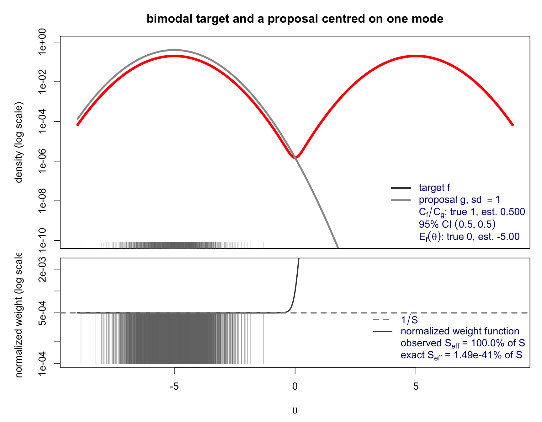
The last two legend entries are the whole lesson. The observed effective sample size is a statistic of the weights that actually appeared, and it reports near-perfect efficiency. The exact effective fraction \(1/E_{g}(w^{2})\), available here in closed form because both densities are Gaussian mixtures, is smaller by some forty orders of magnitude. At \(\sigma=1\) the variance is finite, so the central limit theorem does apply and the estimator is consistent; it would simply need \(S\) of order \(10^{43}\) before its sampling distribution resembled a normal one. Finiteness of the variance is itself fragile: the exact second moment diverges once \(2-\sigma^{-2}\le 0\), that is for every \(\sigma\le 1/\sqrt{2}\).
There is a shinylive app to illustrate how importance sampling can fail without warning when the proposal is too narrow to cover the target.
The target is a standard Student-\(t_{\nu}\) distribution, with the degrees of freedom \(\nu\) a tuning parameter of the target that controls how heavy its tail is: \(\nu=1\) is the standard Cauchy, and \(\nu\to\infty\) recovers the standard normal. The goal is \(P(c_{1}<X<c_{2})\) for an interval \((c_{1},c_{2})\) — possibly one-sided, \(c_{2}=\infty\) — estimated from draws of a truncated-normal proposal generated by adaptive rejection sampling (ARS).
As in the ARS section of the previous chapter, \(\log\varphi\) is concave, and restricting to \((c_{1},c_{2})\) (or one-sided, \((c_{1},\infty)\)) preserves concavity, so the ars package applies directly: rtnorm_ars() below just hands it the log-density and its derivative, plus the truncation bounds.
## ---------------------------------------------------------------------
##  rtnorm_ars(): draw from N(mu, sigma^2) truncated to (lo, hi) (hi may
##  be Inf) via the ars package. log-phi is concave, so ars() applies
##  directly; x0 gives it three starting abscissae inside (lo, hi), with
##  the rightmost past mu when hi = Inf so the upper piece has negative
##  slope and stays integrable.
## ---------------------------------------------------------------------
rtnorm_ars <- function(n, mu = 0, sigma = 1, lo = 0, hi = Inf) {
    logf   <- function(x) dnorm(x, mu, sigma, log = TRUE)
    fprima <- function(x) -(x - mu) / sigma^2
    if (is.finite(hi)) {
        x0 <- lo + (hi - lo) * c(0.1, 0.5, 0.9)
    } else {
        right <- max(mu, lo) + 3 * sigma
        x0 <- sort(unique(c(lo + 0.1 * sigma, max(lo + 0.2 * sigma, mu + 1e-6), right)))
    }
    ars(n, f = logf, fprima = fprima, x = x0,
        lb = TRUE, xlb = lo, ub = is.finite(hi), xub = if (is.finite(hi)) hi else 0)
}
The ars package is itself available inside the browser — webR fetches it from CRAN’s WebAssembly mirror the first time library(ars) runs — so the interactive app below calls this exact function, not a hand-rolled substitute.
The contrast with the target is the point of the exercise: ARS needs log-concavity, and \(\log f_{t_{\nu}}\) is simply not concave, for any finite \(\nu\) — it is convex out in the tails, and only the limit \(\nu\to\infty\) (the normal) is concave everywhere. So ARS cannot sample the target directly at any finite \(\nu\); the truncated-normal proposal above is a substitute, not a target-side match, which is exactly why the sample needs importance weights at all.
A one-sided tail \((c,\infty)\) is a bad target for this proposal, so consider instead a general interval \((c_{1},c_{2})\), with \(c_{2}=\infty\) allowed as a special case. Let \(g\) be the normalized truncated normal on \((c_{1},c_{2})\) and \(f(x)=f_{t_{\nu}}(x)I(c_{1}<x<c_{2})\). Draw \(X_{1},\dots,X_{S}\sim g\), weight each by \(w(x)=f(x)/g(x)\), and average: \[ \widehat{C} \;=\; \frac{1}{S}\sum_{i=1}^{S} w(X_{i}). \] This is unbiased for \(C_{f}=P(c_{1}<X<c_{2})\) for any \(g\) that is positive wherever \(f\) is — that is the whole mechanism of importance sampling, and it does not care what \(c_{1},c_{2},\mu,\sigma,\nu\) are.
Whether \(\widehat C\) is precise is a different question, governed by \[ \operatorname{Var}_{g}\bigl(w(X)\bigr) \;=\; \int_{c_{1}}^{c_{2}}\frac{f_{t_{\nu}}(x)^{2}}{g(x)}\,dx \;-\; C_{f}^{2} . \] When \(c_{2}\) is finite, \(f\) and \(g\) share the same bounded interval, the ratio \(f/g\) is bounded on it, and the integral is finite — a well-behaved estimator, whatever \(\nu\) is. Send \(c_{2}\to\infty\), though, and the tails stop matching: \(f_{t_{\nu}}(x)^{2}\) decays only polynomially (\(\propto x^{-2(\nu+1)}\)) while \(g\)’s Gaussian tail decays much faster, so the integrand grows without bound and the integral diverges — for every \(\mu,\sigma\) and every finite \(\nu\). The app below lets you flip between the two regimes with a single checkbox, and, as before, \(S_{\text{eff}}\) need not warn you when you have landed in the bad one.
is_t_interval() turns the estimator above into code: draw \(X\) from rtnorm_ars(), form the log-weight \(\log f_{t_\nu}(X) - \log g(X)\), and report \(\widehat C\), its standard error, and \(S_{\text{eff}}\).
## ---------------------------------------------------------------------
##  is_t_interval(): importance-sampling estimate of P(c1 < X < c2) for a
##  standard t_df target, using X ~ N(mu, sigma^2) truncated to (c1, c2)
##  as the proposal.
## ---------------------------------------------------------------------
is_t_interval <- function(S, df, c1, c2, mu, sigma, seed = NULL) {
    if (!is.null(seed)) set.seed(seed)
    X <- rtnorm_ars(S, mu, sigma, c1, c2)

    ## log importance weight  log f_t(x; df) - log g(x),  with g the
    ## normalized truncated normal on (c1, c2)
    lZ   <- log(pnorm(c2, mu, sigma) - pnorm(c1, mu, sigma))
    logw <- dt(X, df, log = TRUE) - (dnorm(X, mu, sigma, log = TRUE) - lZ)

    m    <- max(logw)
    v    <- exp(logw - m)                       # rescaled weights
    Chat <- mean(v) * exp(m)                    # unbiased estimate of P(c1 < X < c2)
    se   <- sd(v) / sqrt(S) * exp(m)            # nominal standard error
    wn   <- v / sum(v)                          # normalized weights

    list(X = X, wn = wn, Chat = Chat, se = se, ess = 1 / sum(wn^2),
         truth = pt(c2, df) - pt(c1, df))
}
Four settings make the point concretely: a finite interval is well-behaved at any \(\nu\), while \(c_{2}=\infty\) reproduces the divergence — badly at \(\nu=1\), but deceptively well at \(\nu=30\), exactly as Table 11.1 shows.
settings <- data.frame(df = c(1, 10, 1, 30), c1 = c(1, 1, 1, 1), c2 = c(3, 3, Inf, Inf))
res <- lapply(seq_len(nrow(settings)), function(i) with(settings[i, ],
    is_t_interval(S = 5000, df = df, c1 = c1, c2 = c2, mu = 0, sigma = 1, seed = 1)))

knitr::kable(data.frame(
    df       = settings$df,
    c1       = settings$c1,
    c2       = ifelse(is.finite(settings$c2), as.character(settings$c2), "Inf"),
    truth    = sapply(res, `[[`, "truth"),
    estimate = sapply(res, `[[`, "Chat"),
    se       = sapply(res, `[[`, "se"),
    ess_pct  = 100 * sapply(res, `[[`, "ess") / 5000
), digits = 4, col.names = c("df", "c1", "c2", "truth", "estimate", "s.e.", "ESS %"))is_t_interval() with S = 5000: a finite c2 is well-behaved at every df, c2 = Inf reproduces the divergent case, badly at df = 1 and only deceptively well at df = 30.
| df | c1 | c2 | truth | estimate | s.e. | ESS % |
|---|---|---|---|---|---|---|
| 1 | 1 | 3 | 0.1476 | 0.1490 | 0.0014 | 68.7656 |
| 10 | 1 | 3 | 0.1638 | 0.1642 | 0.0004 | 96.8918 |
| 1 | 1 | Inf | 0.2500 | 0.1821 | 0.0128 | 3.9146 |
| 30 | 1 | Inf | 0.1627 | 0.1627 | 0.0003 | 98.5371 |
There is a shinylive app to show how the choice of constants and proposal determines whether importance sampling of a Student-\(t\) interval is reliable, by displaying the target, the proposal, and the importance weights.
The quadrature and Laplace-approximation chapters compute the marginal likelihood \(P(y) = \int L(\theta)\pi(\theta)\,d\theta\) of the same conjugate-free Gaussian model — unknown mean \(\mu\) and \(w=\log\sigma^2\), independent normal priors — by a product grid and by a mode-and-Hessian approximation, respectively. Importance sampling offers a third route, and one that comes with a built-in accuracy diagnostic (\(S_{\text{eff}}\)) that neither of the other two methods provides directly.
Take \(g(\mu,w)\) to be the Gaussian approximation to the posterior obtained by a Laplace fit: locate the posterior mode \((\hat\mu,\hat w)\) by optimization, take \(g = N_2\big((\hat\mu,\hat w),\, H^{-1}\big)\) for \(H\) the Hessian of \(-\log[L\pi]\) at the mode, and importance-sample from \(g\) with \(f = L\pi\): \[
\widehat{P(y)} = \frac{1}{S}\sum_{s=1}^S w_s, \qquad
w_s = \frac{L(\theta_s)\pi(\theta_s)}{g(\theta_s)}, \qquad \theta_s \sim g.
\] Because \(g\) is shaped like the posterior near its mode, this is a “good story” proposal by construction — in sharp contrast to sampling directly from the (typically much wider, uninformative) prior, which is exactly the log_marlik_mc function used elsewhere in this book as a naive-Monte-Carlo check: it is importance sampling with \(g = \pi\), and its weights are just the likelihood values \(L(\theta_s)\).
Implementation
log_lik   <- function(x, mu, w) sum(dnorm(x, mu, exp(w / 2), log = TRUE))
log_prior <- function(mu, w, mu_0, sigma_mu, w_0, sigma_w) {
    dnorm(mu, mu_0, sigma_mu, log = TRUE) + dnorm(w, w_0, sigma_w, log = TRUE)
}
neg_log_post <- function(theta, x, mu_0, sigma_mu, w_0, sigma_w) {
    -log_lik(x, theta[1], theta[2]) -
        log_prior(theta[1], theta[2], mu_0, sigma_mu, w_0, sigma_w)
}

### log density of N(mu, A^{-1}) at every column of a 2 x S matrix of points at once,
### replacing a per-point apply() call with one vectorized quadratic form
log_dmvnorm_batch <- function(Theta, mu, A) {
    Tc <- Theta - mu
    quad <- colSums((A %*% Tc) * Tc)
    0.5 * (-nrow(Theta) * log(2 * pi) + sum(log(svd(A)$d)) - quad)
}

### log marginal likelihood by importance sampling from a Laplace-shaped Gaussian.
### Besides S_eff, attaches "se": the standard error of the *log* estimate,
### sd(v) / (sqrt(S) * mean(v)) for v = exp(lw - max(lw)) -- the delta-method
### transfer of the raw estimator's SE onto the log scale, exactly as used for
### the log estimate in the t-interval app above.
log_marlik_imps <- function(x, mu_0, sigma_mu, w_0, sigma_w, S) {
    fit <- nlm(neg_log_post, c(mean(x), log(stats::var(x))), hessian = TRUE,
               x = x, mu_0 = mu_0, sigma_mu = sigma_mu, w_0 = w_0, sigma_w = sigma_w)
    mu_hat <- fit$estimate; H <- fit$hessian
    L <- t(chol(solve(H)))                        # Sigma = H^{-1} = L L'
    Theta <- L %*% matrix(rnorm(2 * S), 2, S) + mu_hat

    log_g <- log_dmvnorm_batch(Theta, mu_hat, H)
    log_f <- -apply(Theta, 2, neg_log_post, x = x, mu_0 = mu_0, sigma_mu = sigma_mu,
                     w_0 = w_0, sigma_w = sigma_w)
    lw <- log_f - log_g
    m  <- max(lw); v <- exp(lw - m)
    structure(log_sum_exp(lw) - log(S),
              ess = log_ess(lw), se = sd(v) / (sqrt(S) * mean(v)))
}

### log marginal likelihood by naive Monte Carlo from the prior (g = pi): a
### second, independent importance-sampling estimator with an unfavourable g
log_marlik_prior <- function(x, mu_0, sigma_mu, w_0, sigma_w, S) {
    mus <- rnorm(S, mu_0, sigma_mu); ws <- rnorm(S, w_0, sigma_w)
    lw <- vapply(seq_len(S), function(i) log_lik(x, mus[i], ws[i]), numeric(1))
    m  <- max(lw); v <- exp(lw - m)
    structure(log_sum_exp(lw) - log(S),
              ess = log_ess(lw), se = sd(v) / (sqrt(S) * mean(v)))
}

### "truth": log marginal likelihood by a midpoint grid over (mu, w), centred
### and scaled by the Laplace fit. The likelihood term is vectorized over the
### whole mu-grid at once via the sufficient statistic sum((x - mu)^2), so --
### like log_dmvnorm_batch above -- no R-level loop over grid points, or over
### data points beyond the one sum(), is needed.
log_marlik_grid <- function(x, mu_0, sigma_mu, w_0, sigma_w, n_grid = 400, width = 8) {
    n   <- length(x)
    fit <- nlm(neg_log_post, c(mean(x), log(stats::var(x))), hessian = TRUE,
               x = x, mu_0 = mu_0, sigma_mu = sigma_mu, w_0 = w_0, sigma_w = sigma_w)
    se  <- sqrt(diag(solve(fit$hessian)))
    mu_grid <- fit$estimate[1] + seq(-width, width, length.out = n_grid) * se[1]
    w_grid  <- fit$estimate[2] + seq(-width, width, length.out = n_grid) * se[2]

    SS <- sum(x^2) - 2 * mu_grid * sum(x) + n * mu_grid^2   # sum((x - mu)^2)
    log_lik_grid   <- outer(SS, w_grid,
                             function(ss, w) -0.5 * n * log(2 * pi) - n * w / 2 - 0.5 * exp(-w) * ss)
    log_prior_grid <- outer(dnorm(mu_grid, mu_0, sigma_mu, log = TRUE),
                             dnorm(w_grid, w_0, sigma_w, log = TRUE), "+")

    h_mu <- diff(mu_grid[1:2]); h_w <- diff(w_grid[1:2])
    log_sum_exp(as.vector(log_lik_grid + log_prior_grid)) + log(h_mu) + log(h_w)
}
log_marlik_grid() supplies ground truth by quadrature — a midpoint grid over \((\mu,w)\), centred and scaled by the same Laplace fit used for the importance proposal, wide enough (8 posterior SDs each way, on a \(400\times
400\) grid) that refining it further does not move the answer. Comparing both proposals against it in a single run, with a 95% CI built from the standard error of that run, makes the difference between them concrete rather than just asserted.
Results across sample sizes
Both proposals target the same \(f=L\pi\), and the prior is a legitimate proposal for it: every posterior draw has positive prior density, so the support condition holds. The two differ only in how well their shape matches the target’s, and the following table varies the amount of data to make that difference visible.
set.seed(4)
ns <- c(5, 20, 100, 400)
S  <- 2000

## one proposal, one data set: estimate, interval and S_eff as a % of S
summarize_is <- function(fn, x, S) {
    est <- fn(x, 0, 5, 0, 5, S)
    se  <- attr(est, "se")
    c(estimate = sprintf("%.2f", as.numeric(est)),
      ci       = sprintf("(%.2f, %.2f)",
                         as.numeric(est) - 1.96 * se,
                         as.numeric(est) + 1.96 * se),
      ess      = sprintf("%.1f", 100 * attr(est, "ess") / S))
}

merged_tbl <- do.call(rbind, lapply(ns, function(n) {
    x   <- rnorm(n)
    lap <- summarize_is(log_marlik_imps,  x, S)
    pri <- summarize_is(log_marlik_prior, x, S)
    data.frame(n     = n,
               truth = sprintf("%.2f", log_marlik_grid(x, 0, 5, 0, 5)),
               lap_estimate = lap[["estimate"]],
               lap_ci       = lap[["ci"]],
               lap_ess      = lap[["ess"]],
               pri_estimate = pri[["estimate"]],
               pri_ci       = pri[["ci"]],
               pri_ess      = pri[["ess"]],
               row.names    = NULL)
}))

## repeated names are intentional: the proposal is carried by the banner
names(merged_tbl) <- c("n", "truth",
                       "estimate", "95% CI", "ESS %",
                       "estimate", "95% CI", "ESS %")

tinytable::tt(merged_tbl) |>
    tinytable::group_tt(j = list("Laplace-shaped proposal" = 3:5,
"prior sampling" = 6:8))| Laplace-shaped proposal | prior sampling | ||||||
|---|---|---|---|---|---|---|---|
| n | truth | estimate | 95% CI | ESS % | estimate | 95% CI | ESS % |
| 5 | -10.09 | -10.16 | (-10.21, -10.11) | 43.3 | -10.00 | (-10.31, -9.69) | 1.9 |
| 20 | -37.29 | -37.31 | (-37.33, -37.29) | 84.9 | -36.86 | (-37.32, -36.40) | 0.9 |
| 100 | -153.02 | -153.01 | (-153.02, -153.01) | 96.3 | -153.94 | (-155.12, -152.76) | 0.1 |
| 400 | -531.18 | -531.18 | (-531.18, -531.18) | 99.2 | -534.74 | (-536.43, -533.05) | 0.1 |
The Laplace-shaped proposal re-centers and re-scales itself around the posterior mode for every data set. Its interval stays tight and centred on the truth at every \(n\), and \(S_{\text{eff}}\) stays close to the nominal \(S\): a second-order approximation to the posterior is evidently a good match to it. Prior sampling degrades monotonically. The posterior concentrates at rate \(n^{-1/2}\) while the prior does not move, so the fraction of prior mass lying where the likelihood is appreciable shrinks with \(n\), the weights become ever more concentrated on a handful of draws, and \(S_{\text{eff}}\) falls to a small fraction of one percent. Its interval may still cover the truth, but it is only as trustworthy as those few draws happen to be from one run to the next.
This is the marginal-likelihood instance of the lesson drawn from the missed-mode example: a fixed, data-independent proposal becomes an increasingly poor match to a target that concentrates as data accumulate, and only a proposal that adapts to the target avoids the resulting collapse in efficiency. Note also the contrast in how the two failures announce themselves. Prior sampling fails noisily — \(S_{\text{eff}}\) reports the collapse directly, which is exactly what the diagnostic is built to catch. The earlier tail examples failed silently, with \(S_{\text{eff}}\) near its nominal value while the estimate was badly wrong, because there the weights were uniform among the draws actually observed and the trouble lay entirely outside the region the proposal ever visited.
There is a shinylive app to show how the distribution of the importance weights reveals the quality of a proposal for estimating a marginal likelihood, comparing a Laplace-shaped proposal with the prior.
The two fundamental estimators from Fundamental Estimators were stated for a generic unnormalized target \(f\), but nothing in their derivation assumes \(f\) is a likelihood or a density. Taking \(f(\theta) = \mathbf 1_A(\theta)\), the indicator of a region \(A \subset \mathbb R^2\), collapses \(C_f = \int f(\theta)\,d\theta\) to \(\text{Area}(A)\), and the ratio-of-normalizing-constants estimator \(\widehat{C_f/C_g} = \frac1S\sum_s w_s\) becomes an importance-sampling estimator of that area. When \(g\) is uniform on a bounding box, this is exactly the “throw darts and count hits” trick used earlier to estimate \(\pi\) as the area of a circle — importance sampling only starts to matter once the region is irregular, or small relative to its bounding box, so that the choice of \(g\) affects how many of the \(S\) draws actually land somewhere useful.
Consider a region built by a Boolean combination of two disks — a crescent \(A = D_1 \setminus D_2\), where \(D_1\) is the unit disk centred at the origin and \(D_2\) is a disk of radius \(r_2 = 0.9\) centred at \((d, 0)\) with \(d = 0.3\), overlapping most of \(D_1\). This is a constructive solid geometry (CSG) shape: testing whether a point lies in \(A\) is a one-line computation, but the area of \(A\) itself has no elementary formula once more than a couple of primitives are combined this way — exactly the situation CAD and engineering software face after a handful of Boolean operations on solids. Two circles are simple enough that a closed form still exists, from the standard circle-intersection formula; it is kept here only to check the Monte Carlo estimates against ground truth.
r1 <- 1; r2 <- 0.9; d <- 0.3
in_A <- function(x, y) (x^2 + y^2 <= r1^2) & ((x - d)^2 + y^2 > r2^2)

### exact area of A, from the circle-circle intersection formula; used only
### to check the Monte Carlo estimates below
circle_intersection_area <- function(r1, r2, d) {
    r1^2 * acos((d^2 + r1^2 - r2^2) / (2 * d * r1)) +
    r2^2 * acos((d^2 + r2^2 - r1^2) / (2 * d * r2)) -
    0.5 * sqrt((-d + r1 + r2) * (d + r1 - r2) * (d - r1 + r2) * (d + r1 + r2))
}
area_true <- pi * r1^2 - circle_intersection_area(r1, r2, d)

### bounding box for the naive proposal: generous, with no attempt to hug A
xlim <- c(-2, 2); ylim <- c(-2, 2)

### importance-sampling estimate of Area(A) under one of two proposals:
### "box" samples uniformly from the bounding box; "disk" samples uniformly
### from D1, which is known to contain A even though A itself is not known
### in closed form
crescent_is <- function(proposal, S, seed) {
    set.seed(seed)
    if (proposal == "box") {
        x <- runif(S, xlim[1], xlim[2]); y <- runif(S, ylim[1], ylim[2])
        g <- 1 / ((xlim[2] - xlim[1]) * (ylim[2] - ylim[1]))
    } else {
        rr <- r1 * sqrt(runif(S)); th <- runif(S, 0, 2 * pi)
        x <- rr * cos(th); y <- rr * sin(th)
        g <- 1 / (pi * r1^2)
    }
    w <- in_A(x, y) / g
    list(x = x, y = y, hit = in_A(x, y),
         estimate = mean(w), me = 1.96 * sd(w) / sqrt(S), ess = ess(w))
}res_box_vis <- crescent_is("box", 1500, seed = 1)
res_disk_vis <- crescent_is("disk", 1500, seed = 1)
theta_seq <- seq(0, 2 * pi, length.out = 200)
par(mfrow = c(1, 2))
plot(res_box_vis$x, res_box_vis$y, asp = 1, pch = 20,
col = ifelse(res_box_vis$hit, "steelblue", "tomato"),
xlab = "x", ylab = "y",
main = paste(sum(res_box_vis$hit), "of 1500 hit A (box)"))
rect(xlim[1], ylim[1], xlim[2], ylim[2], border = "black", lwd = 2)
lines(r1 * cos(theta_seq), r1 * sin(theta_seq), lwd = 2)
lines(d + r2 * cos(theta_seq), r2 * sin(theta_seq), lwd = 2)
plot(res_disk_vis$x, res_disk_vis$y, asp = 1, pch = 20,
col = ifelse(res_disk_vis$hit, "steelblue", "tomato"),
xlab = "x", ylab = "y", xlim = xlim, ylim = ylim,
main = paste(sum(res_disk_vis$hit), "of 1500 hit A (disk)"))
lines(r1 * cos(theta_seq), r1 * sin(theta_seq), lwd = 2)
lines(d + r2 * cos(theta_seq), r2 * sin(theta_seq), lwd = 2)
par(mfrow = c(1, 1))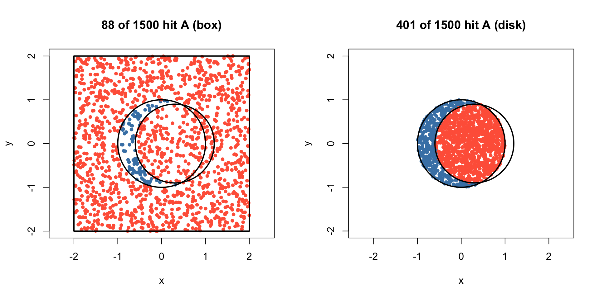
S <- 5000
res_box  <- crescent_is("box",  S, seed = 1)
res_disk <- crescent_is("disk", S, seed = 1)

knitr::kable(data.frame(
    proposal = c("Bounding box (naive)", "Disk $D_1$ (importance)"),
    truth    = rep(area_true, 2),
    estimate = c(res_box$estimate, res_disk$estimate),
    ME      = c(res_box$me, res_disk$me),
    ess_pct  = 100 * c(res_box$ess, res_disk$ess) / S
), digits = 4, col.names = c("Proposal $g$", "True area", "Estimate", "M.E.", "ESS %"))| Proposal \(g\) | True area | Estimate | M.E. | ESS % |
|---|---|---|---|---|
| Bounding box (naive) | 0.8984 | 0.9056 | 0.1025 | 5.66 |
| Disk \(D_1\) (importance) | 0.8984 | 0.8891 | 0.0392 | 28.30 |
Both rows of Table 11.3 are unbiased for the true area — importance sampling never needed to know \(A\)’s exact shape, only a proposal whose support covers it. What changes is efficiency: the box proposal’s effective sample size is under 6% of \(S\), because most darts land outside \(D_1\) entirely and carry weight zero, while the disk proposal’s effective sample size is close to 28% of \(S\) — five times larger, since every draw at least lands in \(D_1\) and only the ones also landing in \(D_2\) are wasted. The standard error falls by roughly the square root of that factor. Unlike Figure 11.1, no bias is at stake here — a bounding box that is too generous costs precision, not correctness — but the lesson is the same: match the proposal to where the target actually lives.
Statistical physics supplies a second reading of the same estimator. A system with energy \(U(x)\) at inverse temperature \(\beta\) has partition function and free energy \[ Z(\beta) = \int e^{-\beta U(x)}\,dx, \qquad F(\beta) = -\frac{1}{\beta}\log Z(\beta). \] \(e^{-\beta U(x)}/Z(\beta)\) is the Boltzmann distribution at temperature \(1/\beta\): large \(\beta\) (low temperature) concentrates mass where \(U\) is small, small \(\beta\) (high temperature) spreads it out.
To move between two temperatures, importance-sample from \(g(x)=e^{-\beta_0 U(x)}\) to \(f(x) = e^{-\beta_1 U(x)}\). The weight is \(w(x) = f(x)/g(x)=e^{-(\beta_1-\beta_0)U(x)}\), and the ratio-of-normalizing-constants estimator from the start of the chapter reads \[ \frac{Z(\beta_1)}{Z(\beta_0)} = E_{\beta_0}\!\left[e^{-(\beta_1-\beta_0)U(x)}\right], \] an expectation under the \(\beta_0\)-tempered distribution.
Set \(U(\theta) = -\log L(\theta)\). Then \(\beta=0\) gives \(e^{-\beta U}\propto
1\) — up to normalization the prior, taking \(g=\pi(\theta)\) — and \(\beta=1\) gives \(e^{-U}=L(\theta)\), so \(f=L(\theta)\pi(\theta)\) is the (unnormalized) posterior. The ratio \(Z(1)/Z(0)\) is exactly the marginal likelihood \(C_f/C_g\) of the previous section: \[
P(y) = \frac{C_f}{C_g} = E_\pi\!\big[L(\theta)\big] \approx \frac1S\sum_{s=1}^S L(\theta_s), \qquad \theta_s\sim\pi,
\] and \(-\log P(y)\) is, in this language, the free energy of the posterior at \(\beta=1\). This is not a new estimator — it is log_marlik_prior() from above, rederived from a different starting point. The physics vocabulary just names the failure mode precisely: jumping straight from \(\beta=0\) to \(\beta=1\) asks one importance-sampling step to bridge the entire temperature range in a single move, and the wider the prior is relative to the likelihood, the more that one jump resembles the badly matched proposals seen earlier in this chapter.
The fix follows from the algebra of the ratio itself. Chaining intermediate temperatures \(\beta_0=0<\beta_1<\dots<\beta_K=1\), \[ \frac{Z(1)}{Z(0)} = \prod_{k=1}^K \frac{Z(\beta_k)}{Z(\beta_{k-1})}, \qquad \log Z(1)-\log Z(0) = \sum_{k=1}^K \log\frac{Z(\beta_k)}{Z(\beta_{k-1})}, \] and each factor is its own small importance-sampling problem: sample from the tempered distribution at \(\beta_{k-1}\), weight by \(e^{-(\beta_k-\beta_{k-1})U(\theta)}\). If the temperatures are close enough together, \(g_{\beta_{k-1}}\) and \(f_{\beta_k}\) nearly coincide and every step is a good-story proposal with near-constant weights — the same principle as building an envelope from many well-fitting pieces rather than one loose one. This chain of intermediate distributions is a stepping-stones estimator (a discretization of thermodynamic integration, and the same schedule idea behind simulated annealing and parallel tempering).
Cross-validation asks how well a model predicts observations it was not fitted to. The Bayesian version of a single leave-one-out fold is the leave-one-out predictive density \[ p(y_i\mid y_{-i}) = \int p(y_i\mid\theta)\,p(\theta\mid y_{-i})\,d\theta, \] the posterior predictive density for \(y_i\) under the posterior that never saw \(y_i\). Summed in log over \(i=1,\dots,n\), these give the expected log pointwise predictive density, a standard measure of a model’s out-of-sample fit. Computed directly it requires refitting the model \(n\) times — one full posterior per left-out observation — exactly the cost importance sampling is suited to avoid.
Take \(g(\theta)=p(\theta\mid y)\), the full posterior — already available from a single fit — as the proposal, and target the leave-one-out posterior \(f(\theta)=p(\theta\mid y_{-i})\). Since \(p(\theta\mid y)\propto p(y_i\mid\theta)\,p(\theta\mid y_{-i})\), \[ f(\theta) = p(\theta\mid y_{-i}) \;\propto\; \frac{p(\theta\mid y)}{p(y_i\mid\theta)}, \qquad w_i(\theta) = \frac{f(\theta)}{g(\theta)} \;\propto\; \frac{1}{p(y_i\mid\theta)}. \] Reusing the self-normalized estimator from the start of the chapter with \(a(\theta)=p(y_i\mid\theta)\), \[ \widehat{p(y_i\mid y_{-i})} = \frac{\sum_{s} p(y_i\mid\theta_s)\,w_i(\theta_s)}{\sum_s w_i(\theta_s)} = \frac{\sum_s p(y_i\mid\theta_s)/p(y_i\mid\theta_s)}{\sum_s 1/p(y_i\mid\theta_s)} = \frac{S}{\sum_{s=1}^S 1/p(y_i\mid\theta_s)}, \] the harmonic mean of the likelihood contributions \(p(y_i\mid\theta_s)\) over draws from the full posterior (Gelfand, Dey & Chang, 1992) — one weighted average per left-out observation, all reusing the same \(S\) posterior draws from the single original fit.