Let \(Y\) denote the observed data and \(\theta\) the parameter, with likelihood \(L(\theta) = P(Y \mid \theta)\). In many models this quantity is itself an integral (or sum) over latent or missing data \(Z\):
The integral is what makes direct maximization awkward: it destroys the product structure that would otherwise make the log-likelihood a sum of simple terms. The EM algorithm avoids it by working with the complete-data likelihood, which retains that structure, and correcting for the fact that \(Z\) is unobserved.
Table 6.1: Fixes the notation for the observed-data and complete-data likelihoods used throughout the chapter. Observed and complete likelihoods
\(Q\) is an average of\(\ell_{\text{comp}}(\theta; Y, Z)\) over \(P(Z \mid Y, \hat\theta^{(t)})\). It is not\(\ell_{\text{comp}}\!\left(\theta; Y, E(Z \mid Y, \hat\theta^{(t)})\right)\) — that is, EM is not “fill in the missing values with their expectations and maximize”. The two coincide only when \(\ell_{\text{comp}}\) happens to be linear in \(Z\), which is true in both examples of this chapter and false in general.
6.1.3\(Q\) as an average of complete log-likelihoods
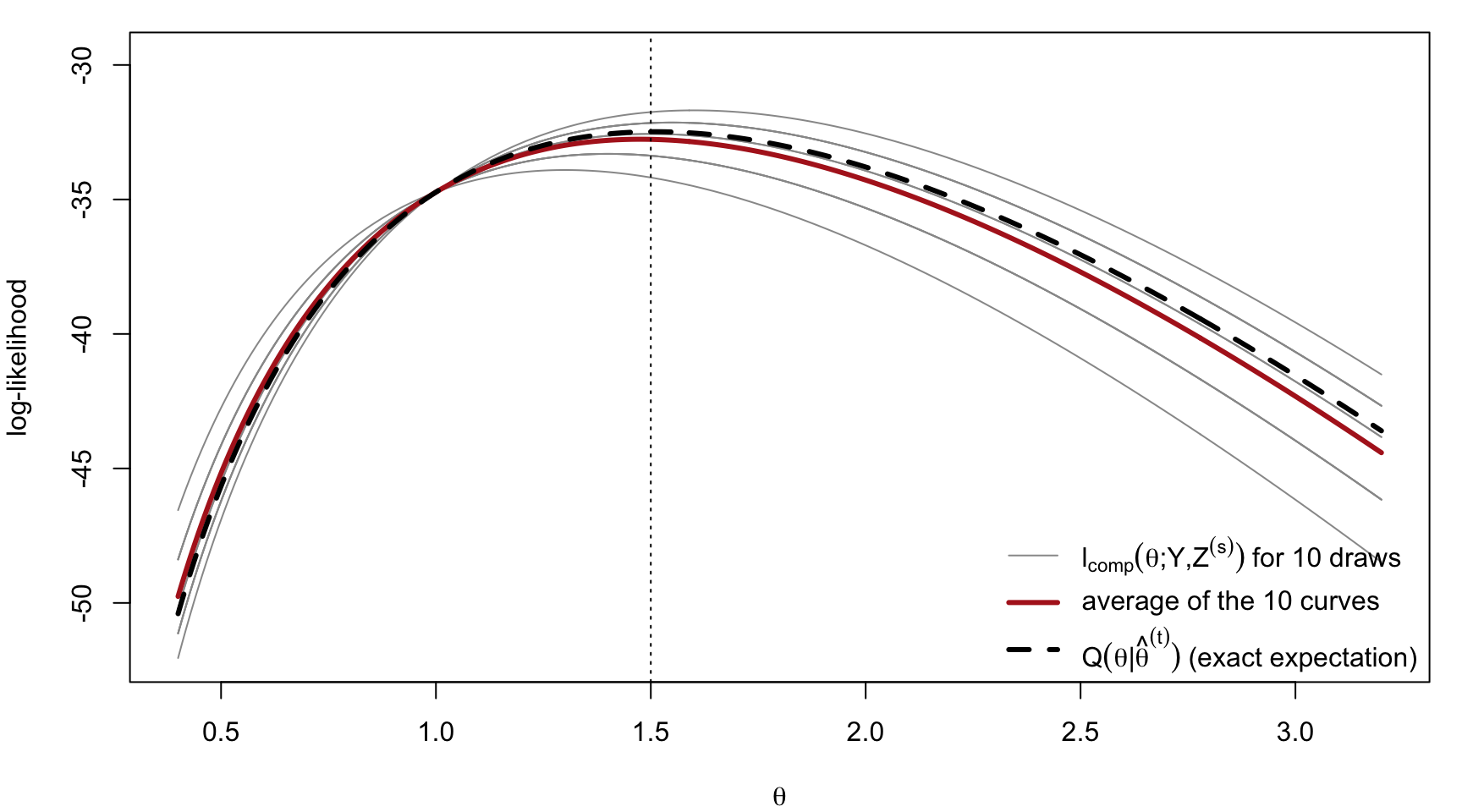
Fix \(\hat\theta^{(t)}\). Each draw \(Z^{(s)} \sim P(Z \mid Y, \hat\theta^{(t)})\) gives one curve \(\ell_{\text{comp}}(\theta; Y, Z^{(s)})\), and \(Q(\theta \mid \hat\theta^{(t)})\) is their expectation. The figure uses the censored Poisson model of Section 6.3 with \(\lambda^{(t)} = 1.5\).
Figure 6.1: Illustrates the \(Q\) function of the EM algorithm as the expectation of the complete-data log-likelihood over the unobserved data, approximated here by averaging simulated completions. Ten complete-data log-likelihood curves, their average, and the exact \(Q\) function.
6.1.4\(Q\) functions as tangent lower bounds
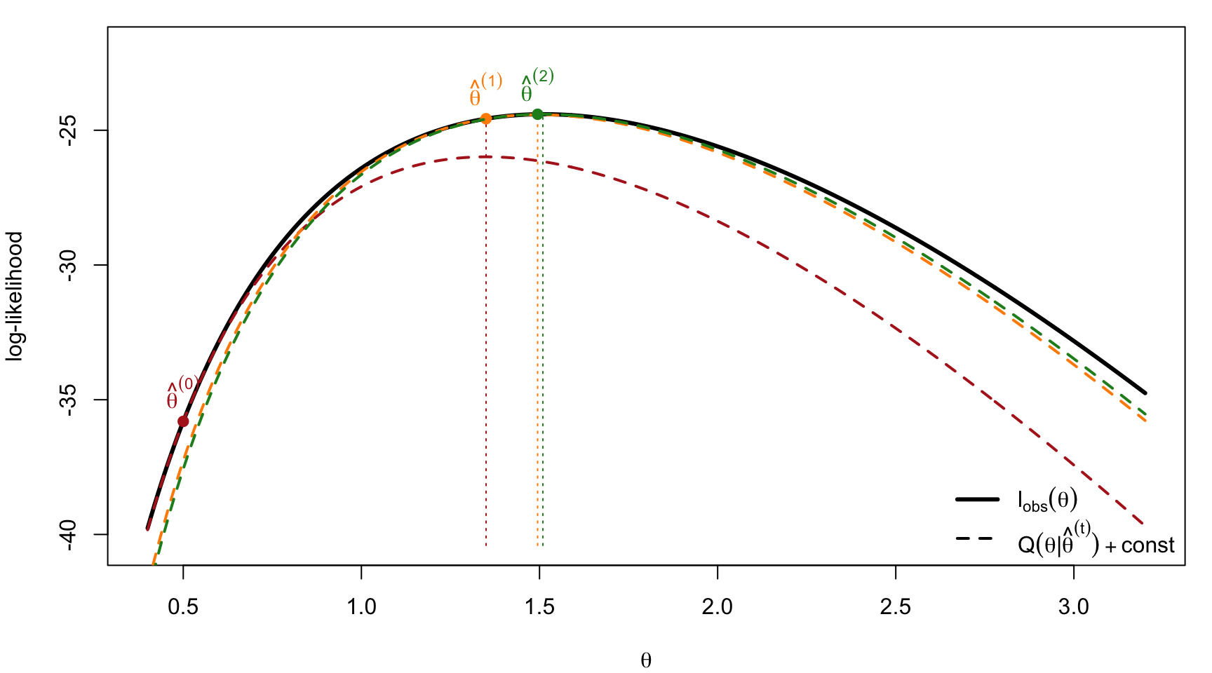
The geometric picture that explains why EM works: each \(Q(\cdot \mid \hat\theta^{(t)})\), shifted by a constant, lies below\(\ell_{\text{obs}}\) and touches it at \(\hat\theta^{(t)}\). Maximizing the bound therefore moves uphill on \(\ell_{\text{obs}}\) itself.
Code
lo <-sapply(lam, lobs); top <-max(lo)par(mar =c(4, 4, 1, 1))plot(lam, lo, type ="l", lwd =3, xlab =expression(theta),ylab ="log-likelihood", ylim =c(top -16, top +2.5))lt <-0.5; cols <-c("firebrick", "darkorange", "forestgreen")for (k in1:3) { shift <-lobs(lt) -Qfun(lt, lt) # make Q touch l_obs at theta^(t)lines(lam, sapply(lam, Qfun, lt = lt) + shift, col = cols[k], lwd =2, lty =2)points(lt, lobs(lt), pch =19, col = cols[k]) lt_new <- (sum(yobs_d) + ncen_d * lt / (1+ lt)) / n_d # M-stepsegments(lt_new, top -16, lt_new, lobs(lt_new), col = cols[k], lty =3)text(lt, lobs(lt), bquote(hat(theta)^(.(k -1))), pos =3, col = cols[k], xpd =NA) lt <- lt_new}legend("bottomright", bty ="n", lwd =c(3, 2), lty =c(1, 2),legend =c(expression(l[obs](theta)),expression(Q(theta*"|"*hat(theta)^(t)) +"const")))
Figure 6.2: Illustrates why EM increases the likelihood: each iteration maximizes a lower bound that touches the observed log-likelihood at the current estimate. Three EM iterations viewed as successive tangent minorants of the observed log-likelihood.
6.1.5 The ascending property
Write \(h(Y, Z \mid \theta) = P(Y, Z \mid \theta)\), \(g(Y \mid \theta) = \int h(Y, Z \mid \theta) \, dZ\), and \(K(Z \mid Y, \theta) = h / g\).
NoteTheorem
\(\ell_{\text{obs}}\!\left(\hat\theta^{(t+1)}\right) \ \ge\ \ell_{\text{obs}}\!\left(\hat\theta^{(t)}\right)\) at every iteration.
Key identity. Since \(\log g(Y \mid \theta) = \log h(Y, Z \mid \theta) - \log K(Z \mid Y, \theta)\) holds for every \(Z\), taking \(E_{Z \mid Y, \theta_0}\) of both sides gives, for any \(\theta_0\),
\[
\ell_{\text{obs}}(\theta)
= \underbrace{E_{Z \mid Y, \theta_0}\!\left[\log h(Y, Z \mid \theta)\right]}_{Q(\theta \mid \theta_0)}
- \underbrace{E_{Z \mid Y, \theta_0}\!\left[\log K(Z \mid Y, \theta)\right]}_{H(\theta \mid \theta_0)} .
\]
The left side does not depend on \(Z\), so the expectation leaves it unchanged; this is the whole content of the step.
Proof. Set \(\theta_0 = \hat\theta^{(t)}\) and subtract the identity evaluated at \(\theta = \hat\theta^{(t)}\) from the one evaluated at \(\theta = \hat\theta^{(t+1)}\):
The \(H\) term. We need \(H(\theta \mid \hat\theta^{(t)}) \le H(\hat\theta^{(t)} \mid \hat\theta^{(t)})\) for every \(\theta\), that is
\[
E_{Z \mid Y, \hat\theta^{(t)}}\!\left[\log \frac{K(Z \mid Y, \theta)}{K(Z \mid Y, \hat\theta^{(t)})}\right] \le 0 .
\]
Because \(\log\) is concave, Jensen’s inequality gives \(E[\log W] \le \log E[W]\), so
\[
\begin{aligned}
E_{Z \mid Y, \hat\theta^{(t)}}\!\left[\log \frac{K(Z \mid Y, \theta)}{K(Z \mid Y, \hat\theta^{(t)})}\right]
&\le \log \int \frac{K(Z \mid Y, \theta)}{K(Z \mid Y, \hat\theta^{(t)})} \, K(Z \mid Y, \hat\theta^{(t)}) \, dZ \\
&= \log \int K(Z \mid Y, \theta) \, dZ = \log 1 = 0 . \qquad \blacksquare
\end{aligned}
\]
The quantity on the left is \(-\mathrm{KL}\!\left(K(\cdot \mid Y, \hat\theta^{(t)}) \,\|\, K(\cdot \mid Y, \theta)\right)\). Note carefully what the theorem does and does not say: the observed likelihood never decreases, but that guarantees convergence only to a stationary point, which may be a local maximum or even a saddle point.
6.1.6 EM as alternating optimization
There is a second formulation that makes the algorithm’s structure clearer and generalizes better. Let \(\tilde P(\cdot)\) be any distribution on the hidden data \(Z\), and define
Both steps of EM are now coordinate ascent on the single function \(F\):
E-step maximizes \(F\) over \(\tilde P\) with \(\theta = \hat\theta^{(t)}\) fixed. Since \(\mathrm{KL} \ge 0\) with equality if and only if \(\tilde P = P(\cdot \mid Y, \hat\theta^{(t)})\), the E-step sets \(\tilde P\) to the conditional distribution of \(Z\).
M-step maximizes \(F\) over \(\theta\) with \(\tilde P\) fixed. The entropy term is free of \(\theta\), so this is \(\arg\max_\theta Q(\theta \mid \hat\theta^{(t)})\).
The ascending property is then immediate: alternating maximization of a single objective cannot decrease it. This view also explains the variational methods used when the E-step is intractable — restrict \(\tilde P\) to a manageable family and accept a bound rather than an equality.
For completeness, \(\mathrm{KL} \ge 0\) follows from \(\log x \le x - 1\):
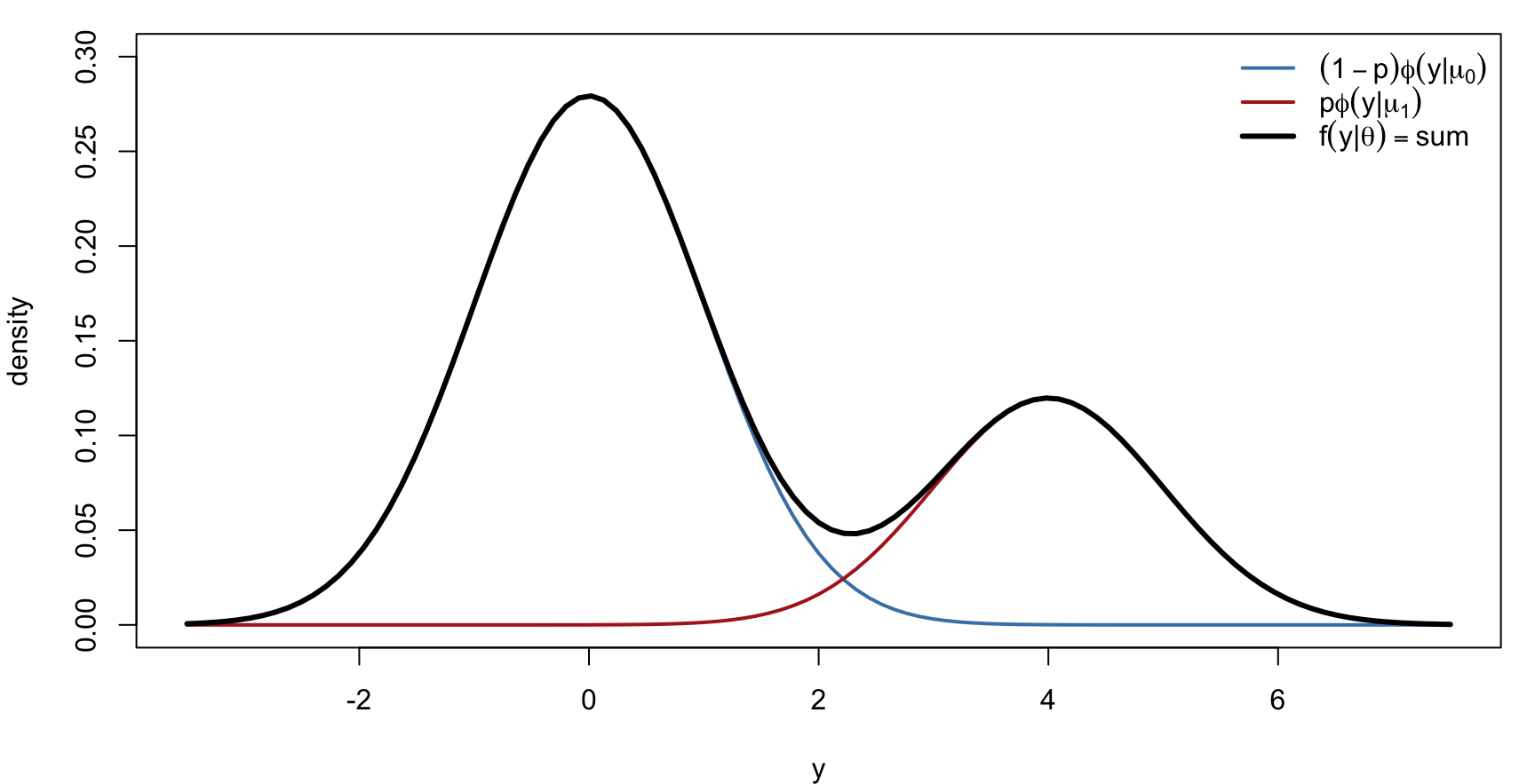
Figure 6.3: Introduces the two-component normal mixture model by showing that its density is the weighted sum of the two component densities. The observed density is a sum of two weighted normal components.
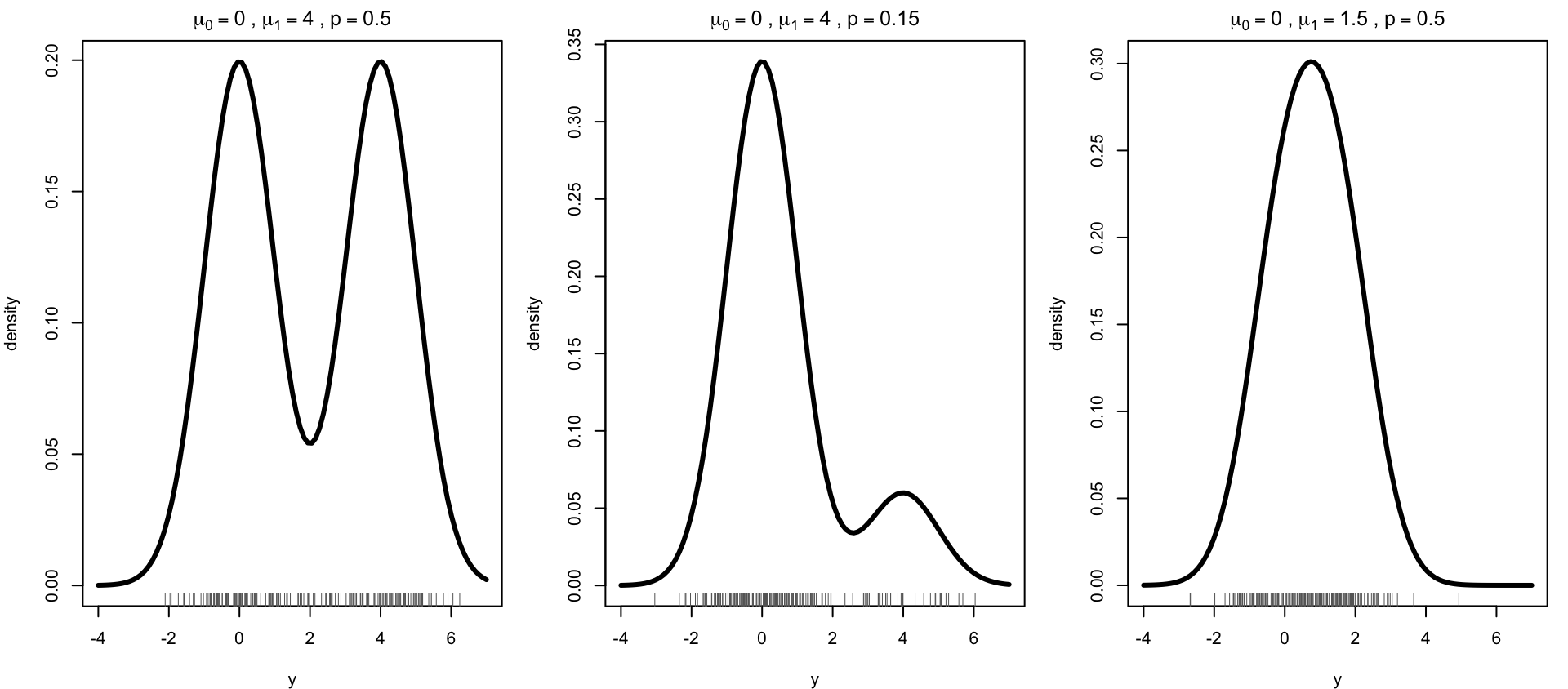
The marginal density may be bimodal or unimodal depending on \(p\) and \(|\mu_1 - \mu_0|\) — a point worth keeping in mind, since the unimodal case is where EM struggles most.
Figure 6.4: Shows that a mixture density can look unimodal or bimodal depending on its parameters, which affects how easily those parameters can be estimated. Separation and mixing proportion determine whether the mixture is visibly bimodal.
\[
\begin{aligned}
\ell_{\text{comp}}(\theta; y, z)
&= \sum_{i=1}^{n}\left[z_i \log p + (1 - z_i)\log(1-p) - \tfrac{1}{2}(y_i - \mu_{z_i})^2\right] + C \\
&= \left(\sum_{i=1}^{n} z_i\right) \log \frac{p}{1-p} + n \log(1-p) \\
&\quad - \frac{1}{2}\sum_{i=1}^{n}\left[z_i (y_i - \mu_1)^2 + (1 - z_i)(y_i - \mu_0)^2\right] + C .
\end{aligned}
\]
Two features drive everything that follows. The expression is linear in each \(z_i\), so the E-step needs only \(E(Z_i \mid y_i, \hat\theta^{(t)})\) rather than the full conditional distribution. And given \(z\), the parameters separate: \(p\) is a Bernoulli proportion while \(\mu_1\) and \(\mu_0\) are group means.
6.2.3 E-step: soft classification
Given \(\hat\theta^{(t)} = (\hat\mu_0^{(t)}, \hat\mu_1^{(t)}, \hat p^{(t)})\), Bayes’ rule gives
Computationally, \(\hat p_i^{(t)}\) must be formed on the log scale. Writing \(a_i = \log \varphi(y_i \mid \hat\mu_1^{(t)}, 1) + \log \hat p^{(t)}\) and \(b_i = \log \varphi(y_i \mid \hat\mu_0^{(t)}, 1) + \log(1 - \hat p^{(t)})\), we have \(\hat p_i^{(t)} = \exp\{a_i - \operatorname{lse}(a_i, b_i)\}\) where \(\operatorname{lse}\) is the log-sum-exp function of the chapter on computer arithmetic. Forming the ratio directly underflows as soon as an observation sits far from both means.
Code
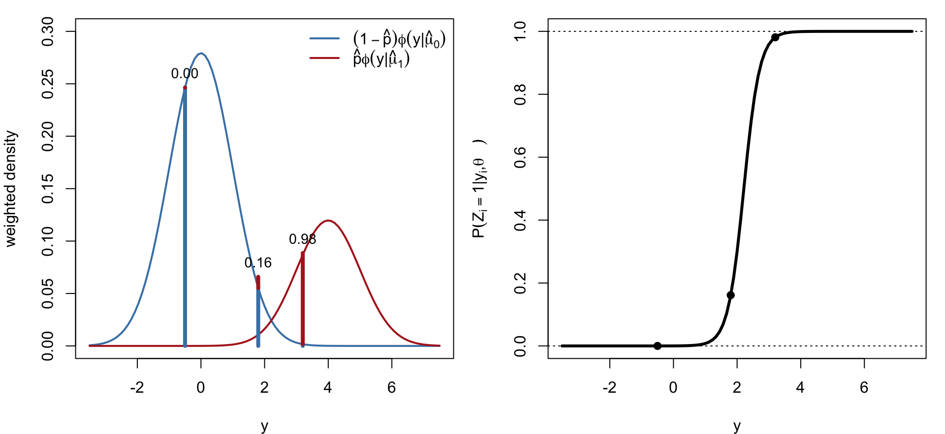
par(mfrow =c(1, 2), mar =c(4, 4, 1, 1)); mu0 <-0; mu1 <-4; p <-0.3f0 <-function(x) (1- p) *dnorm(x, mu0)f1 <-function(x) p *dnorm(x, mu1)curve(f0, -3.5, 7.5, lwd =2, col ="steelblue", ylab ="weighted density",xlab ="y", ylim =c(0, 0.3))curve(f1, add =TRUE, lwd =2, col ="firebrick")yi <-c(-0.5, 1.8, 3.2)for (y in yi) {segments(y, 0, y, f0(y), col ="steelblue", lwd =4)segments(y, f0(y), y, f0(y) +f1(y), col ="firebrick", lwd =4)text(y, f0(y) +f1(y), sprintf("%.2f", f1(y) / (f0(y) +f1(y))), pos =3, cex =0.9)}legend("topright", bty ="n", lwd =2, col =c("steelblue", "firebrick"),legend =c(expression((1-hat(p))*phi(y*"|"*hat(mu)[0])),expression(hat(p)*phi(y*"|"*hat(mu)[1]))))curve(f1(x) / (f0(x) +f1(x)), -3.5, 7.5, lwd =3, xlab ="y",ylab =expression(P(Z[i] ==1*"|"*y[i]*","*hat(theta)^(t))))abline(h =c(0, 1), lty =3); points(yi, f1(yi) / (f0(yi) +f1(yi)), pch =19)
Figure 6.5: Illustrates the E-step of EM for a mixture: the responsibility of a component is the posterior probability that an observation came from it. Left: the responsibility at each \(y_i\) is the red share of the total height. Right: responsibility as a function of \(y\).
6.2.4 M-step: weighted proportions and means
\(Q\) separates into one term in \(p\) and two in \(\mu_1\), \(\mu_0\), each maximized in closed form.
Table 6.2: Derives the M-step updates for the mixture model, showing that each is a weighted version of the complete-data MLE. M-step updates for the two-component mixture
In words: the M-step is the complete-data MLE with each observation split between the two groups in proportion to its soft classification. Return to the E-step with \(\hat\theta^{(t+1)}\) and recompute the responsibilities.
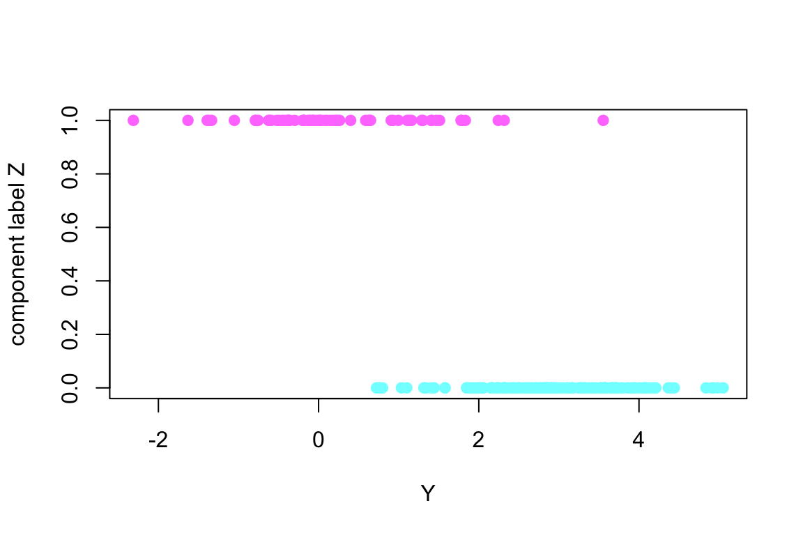
gen_mixnorm <-function(theta, n) { Z <-rbinom(n, 1, theta[1]) Y <-rnorm(n, mean =ifelse(Z ==1, theta[2], theta[3]), sd =1)plot(Y, Z, col =cm.colors(2)[Z +1], pch =19,ylab ="component label Z") Y}set.seed(812)data <-gen_mixnorm(c(0.3, 0, 3), 200)
Figure 6.6: Shows the simulated data used to demonstrate EM for a mixture; the colours reveal the component labels, which are unobserved in practice and must be inferred. Simulated mixture data, coloured by the (normally unobserved) component label.
The monotone increase of the last column is the ascending property in action; it is the single most useful diagnostic when debugging an EM implementation, since any decrease indicates an error in the E- or M-step.
6.2.6 Shinylive App for the EM Algorithm for a Normal Mixture
There is a shinylive app to let you watch the EM algorithm fit a two-component normal mixture, showing how the estimates and the likelihood evolve from iteration to iteration.
6.2.7 Comparison with general-purpose optimizers
EM is not the only way to maximize the observed likelihood. Applying a general-purpose optimizer directly requires attention to the parameter space: \(p\) must lie in \((0,1)\), so we reparameterize with the logit.
Code
neg_loglike_obs <-function(theta, Y) -log_like_obs(theta, Y)### transformed parameterization: ttheta[1] = logit(p)neg_loglike_obs_transf <-function(ttheta, Y) { theta <- ttheta theta[1] <-1/ (1+exp(-ttheta[1]))neg_loglike_obs(theta, Y)}lp0 <-log(0.3/0.7)### Newton-type, untransformed: p can leave (0, 1)try(nlm(neg_loglike_obs, p =c(0.3, 0, 3), Y = data)$estimate)
[1] 0.2968473 0.1131871 2.9203484
Code
try(nlm(neg_loglike_obs, p =c(0.5, -10, 5), Y = data)$estimate)
[1] 5.869764e-06 -1.000004e+01 4.038014e+00
Code
### Newton-type, transformedtry(nlm(neg_loglike_obs_transf, p =c(lp0, 0, 3), Y = data)$estimate)
[1] -0.8623555 0.1131868 2.9203483
Code
try(nlm(neg_loglike_obs_transf, p =c(0, -10, 5), Y = data)$estimate)
[1] -16.604291 -9.996458 2.087049
Code
### Nelder-Meadtry(optim(c(lp0, 0, 3), neg_loglike_obs_transf, Y = data, method ="Nelder-Mead")$par)
[1] -0.8623197 0.1132163 2.9203325
Code
try(optim(c(0, -10, 5), neg_loglike_obs_transf, Y = data, method ="Nelder-Mead")$par)
try(optim(c(0, -10, 5), neg_loglike_obs_transf, Y = data, method ="CG")$par)
[1] -6.090903 -9.998146 2.080878
Applied to the observed log-likelihood, these algorithms are more fragile than EM when the initial values are poorly chosen: the untransformed runs can step outside \(p \in (0,1)\) and produce NaN, and the gradient-based methods can stall in the flat region that a distant start creates. Nelder–Mead is the most stable of the three here, at the cost of many more function evaluations.
Table 6.3: Helps decide between EM and a general-purpose optimizer by listing the strengths and weaknesses of each. EM compared with direct numerical maximization
EM
General optimizer on \(\ell_{\text{obs}}\)
Constraints
Respected automatically by the M-step
Require reparameterization
Monotonicity
Guaranteed; a decrease signals a coding error
None; a bad step can be accepted
Derivatives
None needed
Gradient helpful, Hessian better
Convergence rate
Linear, rate set by the missing information
Superlinear or quadratic near the optimum
Standard errors
Not produced; need Louis’ method or a bootstrap
Hessian available directly
Behaviour from poor starts
Slow but stable
Can fail outright
The last row is the practical trade. EM rarely fails and rarely needs tuning, which is why it dominates in mixture and latent-variable modelling; it is also slow near the optimum and gives no standard errors, which is why a hybrid — EM to get close, then a Newton step to polish and to obtain the Hessian — is common in production code.
6.3 Example 2: Censored Poisson Data
6.3.1 Truncated distributions in brief
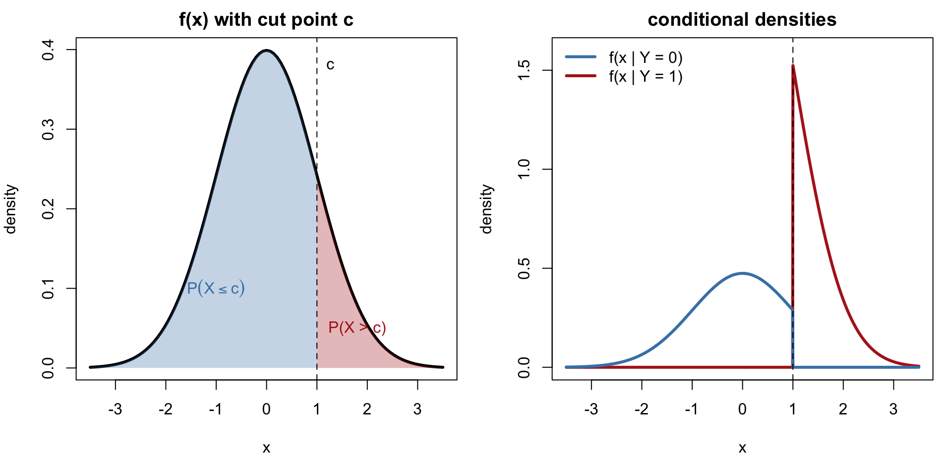
Let \(X \sim f(x)\) and \(Y = I(X > c)\). Then \(Y \sim \text{Bern}\{P(X > c)\}\), and the conditional distribution of \(X\) given \(Y\) is \(f\) restricted to one side of \(c\) and renormalized:
For discrete \(X\) the integrals are sums. This is exactly the distribution the E-step needs when an observation is known only to lie on one side of \(c\).
Figure 6.7: Illustrates the conditional distributions needed in the E-step when an observation is only known to lie on one side of a cut point. A density split at a cut point, and the two renormalized conditional densities.
6.3.2 Data and likelihoods
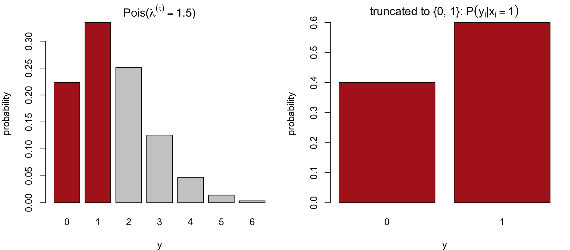
Let \(y_i \overset{iid}{\sim} \text{Pois}(\lambda)\) for \(i = 1, \ldots, n\). The first \(m\) values are observed exactly; for \(i > m\) we know only that \(y_i < 2\), recorded as \(x_i = I(y_i < 2) = 1\).
Observed data: \(y_1, \ldots, y_m\) together with \(x_{m+1} = \cdots = x_n = 1\). Missing: \(y_{m+1}, \ldots, y_n\).
Figure 6.8: Illustrates the E-step for censored Poisson counts: the missing count follows the Poisson distribution restricted to the values consistent with the censoring information. The conditional distribution of a censored count is the Poisson pmf restricted to \(\{0,1\}\) and renormalized.
The update is the ordinary Poisson MLE — the sample mean — with each censored value replaced by its conditional expectation. As warned in the overview, this works only because \(\ell_{\text{comp}}\) is linear in the missing \(y_i\).
6.3.5 Implementation
Code
### observed log-likelihood, up to an additive constant## m : number of exactly observed counts## ybar : their mean## ncen : number of counts known only to be < 2loglik_obs_pois <-function(m, ybar, ncen, lambda) { m * ybar *log(lambda) - (m + ncen) * lambda + ncen *log(1+ lambda)}em_censored_poisson <-function(m, ybar, ncen,lambda0 = (m * ybar + ncen) / (m + ncen),iterations =20) { out <-matrix(NA_real_, iterations +1, 2,dimnames =list(NULL, c("lambda", "log_lik"))) lambda <- lambda0 out[1, ] <-c(lambda, loglik_obs_pois(m, ybar, ncen, lambda))for (i inseq_len(iterations)) { y_mis <- lambda / (1+ lambda) # E-step lambda <- (m * ybar + ncen * y_mis) / (m + ncen) # M-step out[i +1, ] <-c(lambda, loglik_obs_pois(m, ybar, ncen, lambda)) } out}
            m          ncen ybar_observed
   157.000000     43.000000      3.528662
Discarding the censored observations and averaging the rest gives an estimate clearly above the true mean of \(3\): conditioning on \(y \ge 2\) removes the small counts and biases the mean upward. EM recovers them.
Both starting values reach the same limit, and the log-likelihood increases monotonically from each. Note how slowly the run from \(\lambda^{(0)} = 100\) descends at first — a single-parameter illustration of the same slow-drift behaviour seen in the mixture app.
6.3.6 Comparison with general-purpose optimizers
Code
neg_loglik_pois <-function(lambda, m, ybar, ncen) {-loglik_obs_pois(m, ybar, ncen, lambda)}try(nlm(neg_loglik_pois, p = ybar, m = m, ybar = ybar, ncen = ncen)$estimate)
[1] 2.930295
Code
try(nlm(neg_loglik_pois, p =100, m = m, ybar = ybar, ncen = ncen)$estimate)
With one parameter and a smooth concave objective this is an easy problem for any method; the contrast with the mixture example is instructive, since there the multimodality and the constraint on \(p\) were what made the general optimizers fragile.
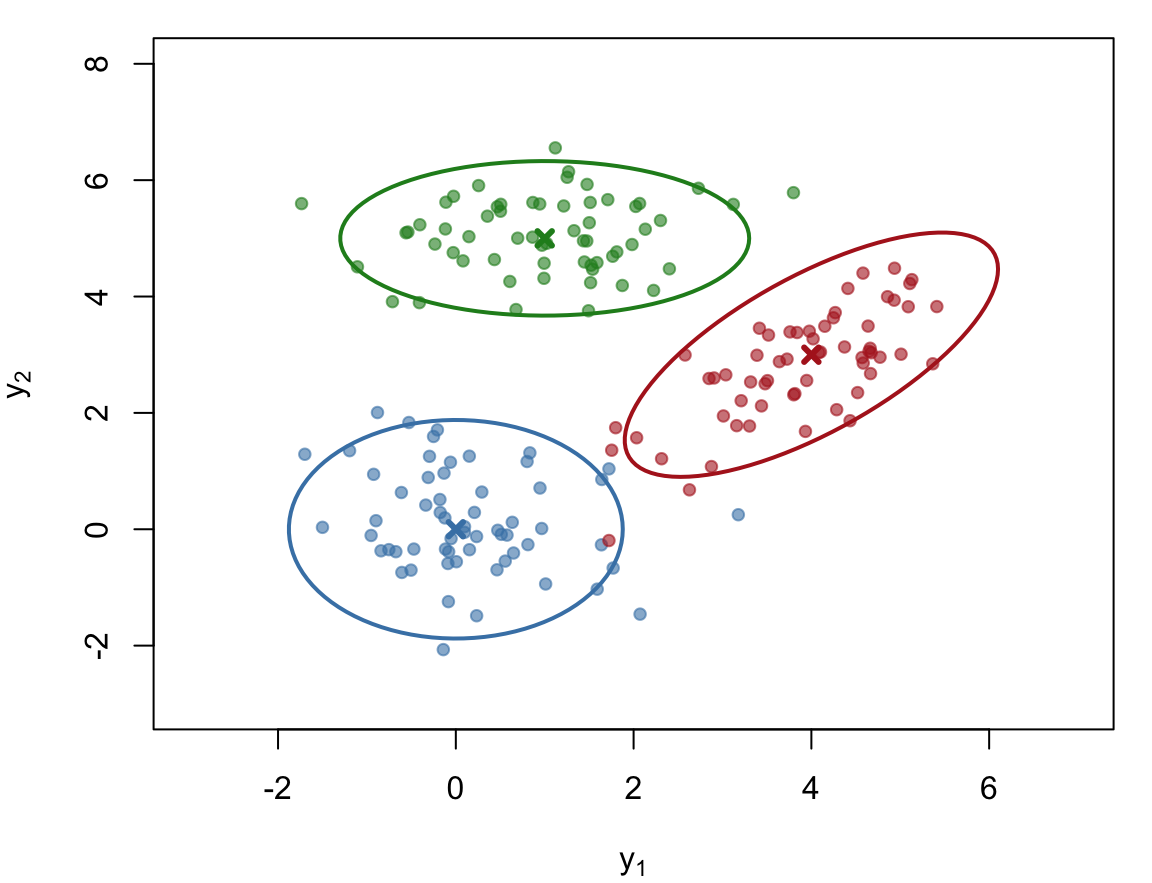
This is the multivariate, \(K\)-component generalization of Section 6.2. The E-step computes soft cluster memberships \(P(Z_i = k \mid y_i, \hat\theta^{(t)})\); the M-step returns weighted means, covariances and proportions. The mclust package implements this with a family of constrained covariance structures.
Figure 6.9: Illustrates model-based clustering, the multivariate extension of the normal mixture model, in which EM assigns observations to clusters of different shapes. Three-component multivariate normal mixture with unequal covariances.
6.4.2 Hidden Markov models
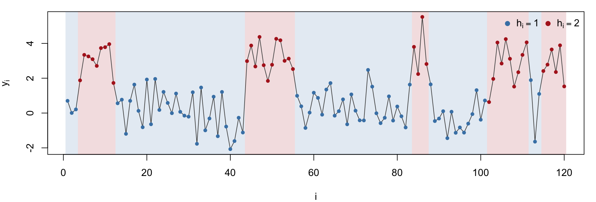
Hidden states \(h_1 \to h_2 \to \cdots \to h_n\) form a Markov chain, and each observation depends only on its own state:
The E-step is the forward–backward algorithm, which computes \(P(h_i \mid y_{1:n}, \hat\theta^{(t)})\) and \(P(h_i, h_{i+1} \mid y_{1:n}, \hat\theta^{(t)})\) without enumerating all \(K^n\) state sequences; the M-step produces weighted transition and emission estimates. The combination is known as the Baum–Welch algorithm, and it is the clearest example of an E-step that is itself a nontrivial computation.
Code
par(mar =c(4, 4, 1, 1)); N <-120Pm <-matrix(c(0.95, 0.05, 0.1, 0.9), 2, byrow =TRUE)h <-integer(N); h[1] <-1for (i in2:N) h[i] <-sample(1:2, 1, prob = Pm[h[i -1], ])yy <-rnorm(N, mean =c(0, 3)[h])plot(yy, type ="n", xlab ="i", ylab =expression(y[i]))r <-rle(h); e <-cumsum(r$lengths); s <-c(1, head(e, -1) +1)rect(s -0.5, par("usr")[3], e +0.5, par("usr")[4],col =adjustcolor(c("steelblue", "firebrick")[r$values], 0.15), border =NA)lines(yy, col ="gray30")points(yy, pch =19, col =c("steelblue", "firebrick")[h], cex =0.7)legend("topright", bty ="n", pch =19, col =c("steelblue", "firebrick"),legend =c(expression(h[i] ==1), expression(h[i] ==2)), horiz =TRUE)
Figure 6.10: Illustrates a hidden Markov model, whose unobserved state sequence generates the data, as a further example to which EM applies. A two-state hidden Markov chain with normal emissions; background shading shows the hidden state.
The E-step uses the fact that \(x_i \mid y_i, \hat\theta^{(t)}\) is normal with closed-form mean and covariance; the M-step is a regression of \(y\) on the expected factors.
Across all these applications the recipe is the same:
Introduce a hidden variable that makes the complete-data model tractable.
E-step: compute the conditional distribution of the hidden data, or just the expected sufficient statistics if \(\ell_{\text{comp}}\) is linear in them.
M-step: compute the complete-data MLE with those expected sufficient statistics in place of the unobserved ones.
The art is entirely in step 1. The same observed-data model often admits several choices of \(Z\), and they lead to EM algorithms with quite different convergence rates — faster when the augmentation adds little information, slower when the missing information is a large fraction of the total.
6.5 Summary
EM maximizes \(\ell_{\text{obs}}\) by alternating between forming \(Q(\theta \mid \hat\theta^{(t)}) = E_{Z \mid Y, \hat\theta^{(t)}}[\ell_{\text{comp}}]\) and maximizing it.
Every iteration weakly increases \(\ell_{\text{obs}}\). Equivalently, EM is coordinate ascent on \(F(\tilde P, \theta) = \ell_{\text{obs}}(\theta) - \mathrm{KL}(\tilde P \,\|\, P(Z \mid Y, \theta))\).
When \(\ell_{\text{comp}}\) is linear in sufficient statistics of \(Z\), the E-step reduces to computing their conditional expectations. Otherwise the full conditional distribution is required, and “plug in the expectation” is wrong.
Convergence is linear, often slow, and only to a stationary point. Run from several starting values and compare the attained log-likelihoods.
Standard errors are not a by-product. Use Louis’ identity, the SEM algorithm, a bootstrap, or a final Newton step.