3  Computer Arithmetic

Author

Longhai Li

Published

September 21, 2026

Statistical computation is arithmetic on a machine that stores every number in a fixed number of binary digits. This chapter describes how integers and real numbers are represented, what goes wrong when a computation exceeds the capacity of that representation (overflow, underflow, and roundoff error), and the standard techniques for writing statistical code that avoids these failures: reordering sums, rewriting formulas, and working on the logarithmic scale.

3.1 Representations of Numbers in Computer

3.1.1 Integers

Every number is a string of digits in boxes, and each box has a place value. In base 10,

10³ 10² 10¹ 10⁰
1 3 4 8

\(1348 = 1\times10^3 + 3\times10^2 + 4\times10^1 + 8\times10^0\)

A computer uses base 2, so each box, called a bit, holds 0 or 1:

2³ 2² 2¹ 2⁰
1 1 0 1

\(1101_2 = 1\times2^3 + 1\times2^2 + 0\times2^1 + 1\times2^0 = 13\)

Everything that follows is a consequence of one fact: the number of boxes is fixed in advance.

An integer is stored in a fixed number of bits, typically 32 or 64. With \(p\) bits the largest unsigned value is obtained by filling every box with 1, \[ \sum_{i=0}^{p-1} 2^i = 2^p - 1 . \] A 4-bit example: the largest storable integer is \(1111_2 = 15\), and \(15 + 1 = 16 = 10000_2\) needs a fifth box that does not exist.

2⁴ 2³ 2² 2¹ 2⁰
1 0 0 0 0

The leading 1 has nowhere to go: integer overflow

To represent negative values, one of the boxes is used as a sign bit, leaving \(p-1\) boxes for the magnitude. With 32 bits, a signed integer \(u\) is \[ u = (-1)^{s}\sum_{i=0}^{30} d_i\,2^i, \qquad s\in\{0,1\}. \] The largest integer has the sign bit \(0\) and the other 31 boxes all equal to \(1\):

sign 2³⁰ 2²⁹ … 2¹ 2⁰
+ 1 1 … 1 1

\(u^{\max} = \sum_{i=0}^{30} 2^i = 2^{31}-1 = 2147483647\)

and the smallest is its negative, \(u^{\min} = -(2^{31}-1)\). When an integer computation leaves this range, R does not wrap around silently, as C does; it returns NA with a warning.

.Machine$integer.max
[1] 2147483647
## Check upper bounds
as.integer(2^31 - 1)                    # maximum valid integer
[1] 2147483647
as.integer(2^31)                        # exceeds limit, returns NA
[1] NA
as.integer(2^31 - 1) + as.integer(1)    # overflows to NA
[1] NA
## Check lower bounds
as.integer(-(2^31 - 1))                 # minimum valid integer
[1] -2147483647
as.integer(-2^31)                       # exceeds lower limit, returns NA
[1] NA

A practical consequence: products of moderately large integers overflow easily. 50000L * 50000L is NA in R, while 50000 * 50000 (double precision) is fine. R converts to double automatically for most arithmetic, so integer overflow is rarely a problem in R code; it is a common one in C, Java, and database systems.

50000L * 50000L
[1] NA
50000 * 50000
[1] 2.5e+09

3.1.2 Floating point numbers

A real number is stored in the form of scientific notation: a sign, a mantissa holding the significant digits, and an exponent: \[ x = (-1)^{s} \times 1.d_1 d_2 \cdots d_p \times 2^{\,e}. \]

sign mantissa (fixed number of digits) exponent
+ 1 . d₁ d₂ … dp ×2^ ± e

More precisely, a floating point number \(x\) is represented by a vector of bits \((s,d_0,\ldots,d_{t-1},e_1,\ldots, e_{k-1})\) as, \[ x = (-1)^s \sum_{i=0}^{t-1}d_i2^{-i}\times 2^{\sum_{i=0}^{k-1}e_i2^i-2^{k-1}}. \]

3.1.3 Zoom Models for Representable Floating Numbers

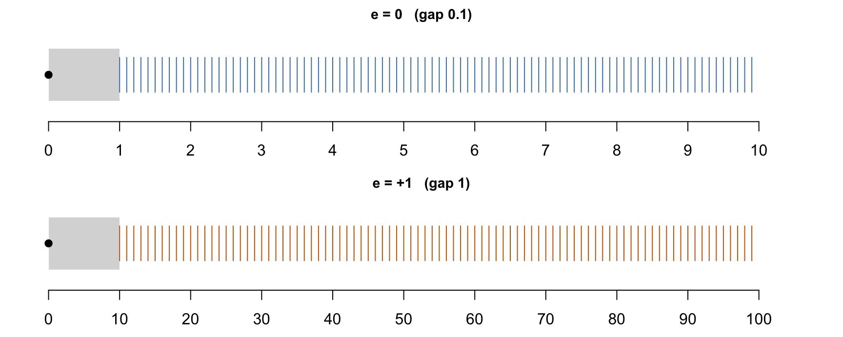
A floating point number is a ruler and a zoom setting. The mantissa is a ruler with a fixed number of equally spaced marks; the exponent stretches it by \(10^{e}\) over \([10^{e}, 10^{e+1})\). Stretching adds no marks, so the marks spread apart as the zoom grows.

3.1.3.1 A toy decimal computer

Each number is stored in six boxes: a sign, a two-digit mantissa \(d_1.d_2\) (\(d_1\in\{1,\ldots,9\}\), \(d_2\in\{0,\ldots,9\}\)), and an exponent made of a sign and one decimal digit, so \(e\in\{-9,\ldots,0,\ldots,+9\}\).

sign 1 10⁻¹ ± exp
+ 3 . 1 ×10^ + 0

\(+3.1\times10^{+0}\), the closest storable value to \(\pi\)

Each of the \(19\) zoom levels is a ruler of \(90\) marks. At the lowest zoom \(e=-9\) the leading digit may also be \(0\) (subnormal numbers), which fills the gap between \(0\) and \(1.0\times10^{-9}\).

zoom \(e\) interval storable numbers gap
\(-9\) (subnormal) \((0, 10^{-9})\) \(0.1\times10^{-9}, \ldots, 0.9\times10^{-9}\) \(10^{-10}\)
\(-9\) \([10^{-9}, 10^{-8})\) \(1.0\times10^{-9}, 1.1\times10^{-9}, \ldots, 9.9\times10^{-9}\) \(10^{-10}\)
\(\vdots\) \(\vdots\) \(\vdots\) \(\vdots\)
\(-1\) \([0.1, 1)\) \(0.10, 0.11, \ldots, 0.99\) \(0.01\)
\(0\) \([1, 10)\) \(1.0, 1.1, \ldots, 9.9\) \(0.1\)
\(+1\) \([10, 100)\) \(10, 11, \ldots, 99\) \(1\)
\(\vdots\) \(\vdots\) \(\vdots\) \(\vdots\)
\(+9\) \([10^{9}, 10^{10})\) \(1.0\times10^{9}, 1.1\times10^{9}, \ldots, 9.9\times10^{9}\) \(10^{8}\)

With both signs, the \(9\) subnormals per sign, and a reserved code for \(0\), the machine stores exactly \(2\times(19\times90+9)+1=3439\) numbers. The \(90\) normal mantissas are listed below; multiplying them by \(10^{e}\), \(e=-9,\ldots,9\), gives every positive normal number.

m <- outer(1:9, 0:9, function(a, b) sprintf("%.1f",a + b / 10))
dimnames(m) <- list(d1 = 1:9, d2 = 0:9)
m
   d2
d1  0     1     2     3     4     5     6     7     8     9    
  1 "1.0" "1.1" "1.2" "1.3" "1.4" "1.5" "1.6" "1.7" "1.8" "1.9"
  2 "2.0" "2.1" "2.2" "2.3" "2.4" "2.5" "2.6" "2.7" "2.8" "2.9"
  3 "3.0" "3.1" "3.2" "3.3" "3.4" "3.5" "3.6" "3.7" "3.8" "3.9"
  4 "4.0" "4.1" "4.2" "4.3" "4.4" "4.5" "4.6" "4.7" "4.8" "4.9"
  5 "5.0" "5.1" "5.2" "5.3" "5.4" "5.5" "5.6" "5.7" "5.8" "5.9"
  6 "6.0" "6.1" "6.2" "6.3" "6.4" "6.5" "6.6" "6.7" "6.8" "6.9"
  7 "7.0" "7.1" "7.2" "7.3" "7.4" "7.5" "7.6" "7.7" "7.8" "7.9"
  8 "8.0" "8.1" "8.2" "8.3" "8.4" "8.5" "8.6" "8.7" "8.8" "8.9"
  9 "9.0" "9.1" "9.2" "9.3" "9.4" "9.5" "9.6" "9.7" "9.8" "9.9"
Figure 3.1: Illustrates how floating-point numbers are spaced on the real line in a toy number system: the gaps between representable numbers grow with magnitude, so precision is relative rather than absolute. Positive numbers at zoom \(e=0\) (top, gap \(0.1\)) and \(e=+1\) (bottom, gap \(1\)). Grey bands hold the crowded marks of all lower zooms (\(e<0\), and \(e\le 0\) in the bottom panel); overflow occurs only far to the right, beyond \(9.9\times10^{9}\).

3.1.3.2 Rounding error and machine epsilon

A real number between two marks is stored as the nearer mark. The three numbers below share the same mantissa boxes and differ only in the exponent, so the absolute error scales with the zoom while the relative error does not.

\(x\) sign 1 10⁻¹ ± exp stored error
\(0.234\) + 2 . 3 ×10^ − 1 \(0.23\) \(0.004\) (1.7%)
\(2.34\) + 2 . 3 ×10^ + 0 \(2.3\) \(0.04\) (1.7%)
\(23.4\) + 2 . 3 ×10^ + 1 \(23\) \(0.4\) (1.7%)

The same rounding occurs in arithmetic. To add, the two numbers are aligned by place value; solid boxes are stored digits, dashed boxes are alignment zeros, and the result keeps only the two boxes starting at its leading digit, so digits to the right (red) are rounded off.

10⁰ 10⁻¹ 10⁻²
1 . 0
+ 0 . 1 0
1 . 1 0

\(1.0 + 0.10 = 1.1 \ne 1.0\)

10⁰ 10⁻¹ 10⁻²
1 . 0
+ 0 . 1 4
1 . 1 4

\(1.0 + 0.14 \to 1.1\)

10¹ 10⁰ 10⁻¹ 10⁻²
1 0 .
+ 0 0 . 4 0
1 0 . 4 0

\(10 + 0.40 \to 10\)

The machine epsilon \(\epsilon\) is the gap next to \(1\), the smallest increment that the second mantissa box can register when added to \(1\); here \(\epsilon = 0.1\) (left). Smaller increments fall into the red box: the digit \(4\) is lost (middle), and at zoom \(e=+1\) the whole addend \(0.40\) is lost (right). Relative to the magnitude, the resolution is about \(\epsilon\) at every zoom.

3.1.3.3 Largest and smallest numbers

sign 1 10⁻¹ ± exp value
largest + 9 . 9 ×10^ + 9 \(9.9\times10^{9}\)
smallest positive + 0 . 1 ×10^ − 9 \(0.1\times10^{-9}\)
largest negative − 0 . 1 ×10^ − 9 \(-0.1\times10^{-9}\)
smallest − 9 . 9 ×10^ + 9 \(-9.9\times10^{9}\)

Largest mantissa with the largest exponent; smallest subnormal mantissa with the smallest exponent

Overflow. A result with magnitude at least \(9.95\times10^{9}\) needs the exponent \(+10\), which the single exponent digit cannot hold, so it is returned as \(\pm\infty\):

10¹⁰ 10⁹ 10⁸
6 0
+ 5 0
1 1 0

\(6.0\times10^{9} + 5.0\times10^{9} = 1.1\times10^{+10} \to \infty\)

sign 1 10⁻¹ ± exp
+ 1 . 1 ×10^ + 10

The exponent \(10\) needs two digits but has one box: overflow

Underflow. A result with magnitude below \(0.05\times10^{-9}\) has no box pattern and is returned as \(0\):

sign 1 10⁻¹ 10⁻² ± exp
+ 0 . 0 1 ×10^ − 9

\((0.1\times10^{-9})\times0.1 = 0.01\times10^{-9} \to 0\): the digit \(1\) falls outside the mantissa

Every later operation treats the underflowed result as exactly zero.

3.1.3.4 Doubles

A double uses the same boxes in base \(2\): \(1\) sign bit, \(11\) exponent bits, and \(52\) mantissa bits after an implicit leading \(1\). The exponent is stored with a bias of \(1023\), so the codes \(1,\ldots,2046\) give \(e\in[-1022, 1023]\); the code \(0\) is reserved for \(0\) and the subnormals, and the code \(2047\) for Inf and NaN.

\[ \newcommand{\bx}[1]{\boxed{\mathtt{#1}}\!} \begin{array}{rccccccl} & \text{sign} & \text{mantissa} & & & \text{exponent} & & \\[4pt] 1 & \bx{+} & {\color{gray}1.}\overbrace{\bx{0}\bx{0}\bx{0}\cdots\bx{0}\bx{0}\bx{0}}^{52\text{ bits}} & & \times2^\wedge & \overbrace{\bx{+}\bx{0}\bx{0}\bx{0}\bx{0}\bx{0}\bx{0}\bx{0}\bx{0}\bx{0}\bx{0}}^{11\text{ bits}} & & \\ +\;\epsilon & \bx{+} & {\color{gray}0.}\bx{0}\bx{0}\bx{0}\cdots\bx{0}\bx{0}\bx{1} & & \times2^\wedge & \bx{+}\bx{0}\bx{0}\bx{0}\bx{0}\bx{0}\bx{0}\bx{0}\bx{0}\bx{0}\bx{0} & & = 2^{-52}\\ \hline 1+\epsilon & \bx{+} & {\color{gray}1.}\bx{0}\bx{0}\bx{0}\cdots\bx{0}\bx{0}\bx{1} & & \times2^\wedge & \bx{+}\bx{0}\bx{0}\bx{0}\bx{0}\bx{0}\bx{0}\bx{0}\bx{0}\bx{0}\bx{0} & & \ne 1\\[20pt] 1 & \bx{+} & {\color{gray}1.}\bx{0}\bx{0}\bx{0}\cdots\bx{0}\bx{0}\bx{0} & & \times2^\wedge & \bx{+}\bx{0}\bx{0}\bx{0}\bx{0}\bx{0}\bx{0}\bx{0}\bx{0}\bx{0}\bx{0} & & \\ +\;\epsilon/2 & \bx{+} & {\color{gray}0.}\bx{0}\bx{0}\bx{0}\cdots\bx{0}\bx{0}\bx{0} & {\color{red}\boxed{\mathtt{1}}} & \times2^\wedge & \bx{+}\bx{0}\bx{0}\bx{0}\bx{0}\bx{0}\bx{0}\bx{0}\bx{0}\bx{0}\bx{0} & & = 2^{-53}\\ \hline 1+\epsilon/2 & \bx{+} & {\color{gray}1.}\bx{0}\bx{0}\bx{0}\cdots\bx{0}\bx{0}\bx{0} & {\color{red}\boxed{\mathtt{1}}} & \times2^\wedge & \bx{+}\bx{0}\bx{0}\bx{0}\bx{0}\bx{0}\bx{0}\bx{0}\bx{0}\bx{0}\bx{0} & & \to 1 \end{array} \]

The machine epsilon is the smallest number that changes \(1\) when added to it: the place value of the last mantissa box at \(e=0\), \(\epsilon = 0.0\cdots01\times2^{0} = 2^{-52}\approx 2.220446\times10^{-16}\). Adding \(\epsilon\) sets that box (top). Adding \(\epsilon/2\) needs a \(53\)rd box (red), which does not exist, so the sum rounds back to \(1\) (bottom; the tie is rounded to the even mantissa).

\[ \begin{array}{rcccl} & \text{mantissa} & & \text{exponent} & \text{value}\\[6pt] \begin{array}{r}\text{largest}\end{array} & {\color{gray}1.}\underbrace{\bx{1}\bx{1}\bx{1}\cdots\bx{1}\bx{1}\bx{1}}_{52\text{ bits}} & \times 2^\wedge & \underbrace{\bx{+}\bx{1}\bx{1}\bx{1}\bx{1}\bx{1}\bx{1}\bx{1}\bx{1}\bx{1}\bx{1}}_{11\text{ bits}} & \begin{array}{l}(2-2^{-52})\times2^{1023}\\\approx 1.797693\times10^{308}\end{array}\\[16pt] \begin{array}{r}\text{smallest}\\\text{normal}\end{array} & {\color{gray}1.}\underbrace{\bx{0}\bx{0}\bx{0}\cdots\bx{0}\bx{0}\bx{0}}_{52\text{ bits}} & \times 2^\wedge & \underbrace{\bx{-}\bx{1}\bx{1}\bx{1}\bx{1}\bx{1}\bx{1}\bx{1}\bx{1}\bx{1}\bx{0}}_{11\text{ bits}} & \begin{array}{l}2^{-1022}\\\approx 2.225074\times10^{-308}\end{array}\\[16pt] \begin{array}{r}\text{smallest}\\\text{positive}\end{array} & {\color{gray}0.}\underbrace{\bx{0}\bx{0}\bx{0}\cdots\bx{0}\bx{0}\bx{1}}_{52\text{ bits}} & \times 2^\wedge & \underbrace{\bx{-}\bx{1}\bx{1}\bx{1}\bx{1}\bx{1}\bx{1}\bx{1}\bx{1}\bx{1}\bx{0}}_{11\text{ bits}} & \begin{array}{l}2^{-1074}\\\approx 4.940656\times10^{-324}\end{array} \end{array} \]

For readability, the picture shows the exponent as a sign box and \(10\) magnitude bits; the hardware stores the same \(11\) bits as the unsigned code \(e+1023\). The grey leading digit is not stored: it is \(1\) for normal doubles and \(0\) for subnormals, which occur only at \(e=-1022\).

  • The largest double has a full mantissa and the largest exponent, \(+1023\).

  • The smallest normal double has mantissa \(1.0\) and the smallest exponent, \(-1022\).

  • The smallest positive double is the subnormal with only the last mantissa box set at \(e=-1022\), i.e. \(2^{-52}\times2^{-1022}=2^{-1074}\).

  • The machine epsilon \(\epsilon=2^{-52}\) is the gap next to \(1\), set by the last mantissa bit. Since the gap in \([2^e, 2^{e+1})\) is \(2^{e-52}\), \(\epsilon\) is also the relative resolution at every magnitude: a double carries about \(15\)–\(16\) significant decimal digits.

  • The largest double has all mantissa bits and all usable exponent bits set to \(1\). Results beyond it overflow to Inf.

  • The smallest normal double has the smallest usable exponent and mantissa \(1.0\). Below it, subnormals fill the gap down to \(2^{-1074}\) with evenly spaced but less precise values; results below half of \(2^{-1074}\) underflow to \(0\).

quantity value R relevance in computing
machine epsilon \(2^{-52}\approx2.2\times10^{-16}\) .Machine$double.eps Doubles cannot be compared exactly (0.1 + 0.2 != 0.3); convergence and equality tests use tolerances such as \(\sqrt{\epsilon}\approx1.5\times10^{-8}\) (all.equal), which is also the usual step size for numerical derivatives
largest double \(\approx1.80\times10^{308}\) .Machine$double.xmax exp(x) overflows for \(x>709.8\); products of large terms such as likelihood ratios or \(n!\) must be computed on the log scale
smallest normal double \(2^{-1022}\approx2.2\times10^{-308}\) .Machine$double.xmin exp(x) leaves the normal range for \(x<-708.4\); a product of many densities falls here, which is why likelihoods are computed as log-likelihoods and sums of exponentials via log-sum-exp
smallest subnormal double \(2^{-1074}\approx4.9\times10^{-324}\) 2^-1074 Last value before underflow to \(0\); subnormals keep few significant bits, so ratios of such values are unreliable
largest consecutive integer \(2^{53}\approx9.0\times10^{15}\) 2^53 Beyond it the gap exceeds \(1\) and integers are skipped; R’s integer type stops even earlier at \(2^{31}-1\), so larger identifiers must be stored as character strings or bit64::integer64

3.1.3.5 Verify in R

c(eps = .Machine$double.eps, xmax = .Machine$double.xmax,
  xmin = .Machine$double.xmin, subnormal = 2^-1074, maxint = 2^53)
                         eps                         xmax 
 2.220446049250313080847e-16 1.797693134862315708145e+308 
                        xmin                    subnormal 
2.225073858507201383090e-308 4.940656458412465441766e-324 
                      maxint 
 9.007199254740992000000e+15 

These are the decimal values in the boxed displays above.

  • eps \(=2^{-52}\) is the place value of the last mantissa box at \(e=0\), the \(\epsilon\) added to \(1\) in the vertical addition.
  • xmax is the “largest” row: a full mantissa with exponent \(+1023\).
  • xmin is the “smallest normal” row: mantissa \(1.0\) with exponent \(-1022\).
  • subnormal is the “smallest positive” row: only the last mantissa box set, with leading digit \(0\) and exponent \(-1022\).
  • maxint \(=2^{53}\) is where the last mantissa box becomes worth \(2\) (see spacing-demo below).
1 + 2^-52 == 1
[1] FALSE
1 + 2^-53 == 1                       # half an epsilon is lost
[1] TRUE
0.1 + 0.2 == 0.3                     # rounding error
[1] FALSE
isTRUE(all.equal(0.1 + 0.2, 0.3))    # test with tolerance sqrt(eps)
[1] TRUE
  • 1 + 2^-52 == 1 is FALSE: the top vertical addition, where \(\epsilon\) sets the last mantissa box and \(1+\epsilon\) is a different double.
  • 1 + 2^-53 == 1 is TRUE: the bottom vertical addition, where \(\epsilon/2\) needs the nonexistent \(53\)rd box (red) and the sum rounds back to \(1\).
  • 0.1 + 0.2 == 0.3 is FALSE: \(0.1\), \(0.2\) and \(0.3\) have infinitely repeating binary mantissas, so each is cut at the \(52\)nd box, and the rounded sum lands on a different mark from the rounded \(0.3\).
  • all.equal(...) is TRUE: it tests equality up to a relative tolerance \(\sqrt{\epsilon}\approx1.5\times10^{-8}\), the safe way to compare doubles.
2 * .Machine$double.xmax             # overflow: Inf
[1] Inf
exp(710)                             # overflow: Inf
[1] Inf
2^-1075                              # underflow: 0
[1] 0
prod(rep(0.01, 200))                 # 1e-400 underflows to 0
[1] 0
sum(log(rep(0.01, 200)))             # the log scale is safe
[1] -921.0340371976157030076
  • 2 * .Machine$double.xmax is Inf: doubling the “largest” row needs exponent \(+1024\), whose code is reserved for Inf, as in the toy \(6.0\times10^{9}+5.0\times10^{9}\).
  • exp(710) is Inf: \(e^{710}\) exceeds xmax \(\approx e^{709.78}\).
  • 2^-1075 is 0: it is half the “smallest positive” row and would need a box beyond the last one; the tie rounds to the even pattern, which is \(0\).
  • prod(rep(0.01, 200)) is 0: the true value \(10^{-400}\) lies below \(2^{-1074}\approx4.9\times10^{-324}\). The same happens to a likelihood built as a product of many densities.
  • sum(log(rep(0.01, 200))) is \(-921.03\): on the log scale the product becomes a sum of moderate numbers, far from both limits.
2^52 + 1 == 2^52                     # gap 1: still distinguishable
[1] FALSE
2^53 + 1 == 2^53                     # gap 2: the +1 is lost
[1] TRUE
format(c(2^53, 2^53 + 1, 2^53 + 2), digits = 17)
[1] "9007199254740992" "9007199254740992" "9007199254740994"
.Machine$integer.max                 # 2^31 - 1
[1] 2147483647
  • 2^52 + 1 == 2^52 is FALSE: at \(e=52\) the last mantissa box is worth \(2^{52-52}=1\), so adding \(1\) sets it, exactly as \(\epsilon\) does at \(e=0\).
  • 2^53 + 1 == 2^53 is TRUE: at \(e=53\) the last box is worth \(2\), so adding \(1\) needs a \(53\)rd box. This is the \(1+\epsilon/2\) addition scaled by \(2^{53}\).
  • format(...) prints 9007199254740992 twice and then 9007199254740994: above \(2^{53}\) only even integers are marks on the ruler.
  • .Machine$integer.max is \(2^{31}-1 = 2147483647\): R’s integer type is \(32\) bits, so integers beyond it, and beyond \(2^{53}\) for doubles, must be stored as character strings or bit64::integer64.

3.2 Methods for Mitigating Rounding Errors

3.2.1 Roundoff errors

The stored result of \(a+b\) (or \(a\times b\), \(a/b\), …) is the nearest representable number to the exact result; digits beyond the mantissa are rounded away, as in the vertical additions above. Each single operation therefore has relative error at most about \(\epsilon\), which is harmless on its own. The concern is when these errors accumulate over many operations or are amplified by the structure of a formula. Two patterns do the amplifying:

  • adding a large + small number, where the small number is partly or wholly rounded away;

  • subtracting large − large nearly equal numbers, where the leading digits cancel and only the roundoff errors survive (catastrophic cancellation).

3.2.2 Computing sums: avoiding large + small

Because the mantissa has finite capacity, a term smaller than half the last box of the large number is lost entirely, as in the addition \(1+\epsilon/2 \to 1\) shown earlier.

Consider \(1.0 + 0.04 + 0.04\) in the toy system, whose exact value is \(1.08\). Evaluated left to right, \((1.0 + 0.04) + 0.04\), each addition rounds back to \(1.0\), so both small terms are lost. Evaluated as \(1.0 + (0.04 + 0.04) = 1.0 + 0.08\), the intermediate sum is exact, and the final addition rounds once, to \(1.1\). Adding the small terms among themselves first commits only one roundoff error, whereas adding them one at a time to the large number commits one per term, and these accumulate.

The following R demonstration makes the same point at machine precision. f2 attempts to add \(2^{-53}\) (half an epsilon) \(2^{13}\) times, but because \(1 + 2^{-53} = 1\) at every single step, the final sum is simply \(1\) instead of \(1 + 2^{-40}\). Grouping the small numbers and adding them together before adding them to the large number (f6s) recovers the correct answer.

The following R demonstration makes the same point at machine precision. f2 attempts to add \(2^{-53}\) (half an epsilon) \(2^{13}\) times, but because \(1 + 2^{-53} = 1\) at every single step, the final sum is simply \(1\) instead of \(1 + 2^{-40}\). Grouping the small numbers and adding them together before adding them to the large number (f6s) recovers the correct answer.

## the target value
f0 <- 1 + 2^(-40)
f0
[1] 1.000000000000909494702
## adding 2^-52 (one epsilon) 2^12 times works: each addition changes the sum
f1 <- 1; i <- 1
while (i <= 2^12) { f1 <- f1 + 2^(-52); i <- i + 1 }
f1
[1] 1.000000000000909494702
## adding 2^-53 (half an epsilon) 2^13 times fails: 1 + 2^-53 rounds to 1 every time
f2 <- 1; i <- 1
while (i <= 2^13) { f2 <- f2 + 2^(-53); i <- i + 1 }
f2
[1] 1
## this difference is not due to number display in R
f0 == f1
[1] TRUE
f0 == f2
[1] FALSE
## R's built-in sum() uses pairwise summation and extended precision
f3 <- sum(c(1, rep(2^(-53), 2^13))); f3
[1] 1
f1 == f3
[1] FALSE
f4 <- sum(c(1, rep(2^(-54), 2^14))); f4
[1] 1
f0 == f4
[1] FALSE
## the fix: accumulate the small numbers first, then add to 1
f6s <- 0; i <- 1
while (i <= 2^14) { f6s <- f6s + 2^(-54); i <- i + 1 }
f6s
[1] 9.09494701772928237915e-13
f6 <- f6s + 1; f6
[1] 1.000000000000909494702
f0 == f6
[1] TRUE

Rules for accurate summation

  • Add numbers of similar magnitude together; when summing terms of very different sizes, add the smallest first (sort ascending).

  • Pairwise summation: sum the two halves of the vector recursively, so that partial sums stay of similar size. R’s sum() uses this together with extended-precision accumulation, which is why sum() beat the naive loop above.

  • Kahan compensated summation: keep track of the part rounded away at each step and add it back at the next step.

x <- c(1, rep(1e-16, 1e4))                 # exact sum is 1 + 1e-12

naive_sum <- function(x) { s <- 0; for (v in x) s <- s + v; s }

kahan_sum <- function(x) {
  s <- 0; c <- 0                            # c holds the running roundoff error
  for (v in x) { y <- v - c; t <- s + y; c <- (t - s) - y; s <- t }
  s }

c(naive   = naive_sum(x) - 1,
  sorted  = naive_sum(sort(x)) - 1,
  kahan   = kahan_sum(x) - 1,
  builtin = sum(x) - 1,
  exact   = 1e-12)
                      naive                      sorted 
0.000000000000000000000e+00 1.000088900582341011614e-12 
                      kahan                     builtin 
1.000088900582341011614e-12 0.000000000000000000000e+00 
                      exact 
9.999999999999999798866e-13 

The naive loop loses every one of the \(10^4\) small terms; sorting recovers most of the answer, and Kahan summation and R’s sum() recover it to full precision.

We can use log() to translate the 52-bit limit into other bases, which tells us at roughly what decimal place precision is lost (about 15 to 16 significant decimal digits).

log(2^(-52))               # base e: about -36
[1] -36.04365338911715355152
1 + exp(-35)
[1] 1.000000000000000666134
1 + exp(-37)               # evaluates to exactly 1
[1] 1
log(2^(-52), base = 10)    # base 10: about -15.7
[1] -15.65355977452702163077
1 + 1e-15 == 1
[1] FALSE
1 + 1e-16 == 1
[1] TRUE

3.2.3 Computing \(e^x\): avoiding large − large

The Taylor series, \[ e^x \approx \sum_{k=0}^{K}\frac{x^k}{k!} = 1 + x + \frac{x^2}{2!} + \frac{x^3}{3!} + \cdots, \] works well for \(x > 0\) but fails for large negative \(x\). For \(x = -20\) the terms alternate in sign and are huge relative to the answer \(e^{-20}\approx 2\times10^{-9}\):

\(k\) 0 1 2 … 20 …
\(x^k/k!\) \(1\) \(-20\) \(200\) … \(4.3\times10^{7}\) …

Each term carries a roundoff error of relative size \(\epsilon \approx 10^{-16}\), i.e. absolute size \(\approx 4\times10^{-9}\) for the largest terms, which is as large as the answer itself. Subtracting nearly equal large numbers leaves only their errors: catastrophic cancellation.

The function fexp below implements the series with a stopping rule based on the relative size of the current term. With debug = TRUE it returns the internal steps rather than the final answer.

library(knitr)

fexp <- function(x, debug = FALSE) {
  i <- 0; expx <- 1; u <- 1
  if (debug) debug_list <- list()
  while (abs(u) > 1e-20 * abs(expx)) {
    i <- i + 1
    u <- u * x / i
    expx <- expx + u
    if (debug) debug_list[[i]] <- c(Step = i, Term_u = u, exp_x = expx)
  }
  if (debug) return(do.call(rbind, debug_list))
  expx
}

test_vals <- c(10, 20, 60, -1, -10, -20, -50)
res1 <- data.frame(x = test_vals, Built_in_Exp = exp(test_vals), Taylor_fexp = sapply(test_vals, fexp))
kable(res1, caption = "Compares a naive Taylor-series implementation of the exponential function with the built-in exp() to show that the series is accurate for positive arguments but fails for negative ones. Built-in exp() versus the naive Taylor series fexp()")
Table 3.1: Compares a naive Taylor-series implementation of the exponential function with the built-in exp() to show that the series is accurate for positive arguments but fails for negative ones. Built-in exp() versus the naive Taylor series fexp()
x Built_in_Exp Taylor_fexp
10 2.202646579480671789497e+04 2.202646579480671061901e+04
20 4.851651954097902774811e+08 4.851651954097902178764e+08
60 1.142007389815684234540e+26 1.142007389815684749937e+26
-1 3.678794411714423340243e-01 3.678794411714424450466e-01
-10 4.539992976248485417315e-05 4.539992962303128097232e-05
-20 2.061153622438600056153e-09 5.621884472130400241374e-09
-50 2.000000000000000097194e-22 1.107293338289196981350e+04

For positive \(x\) the series is accurate to all printed digits. For \(x = -10\) the answer is already off in the fourth digit, for \(x = -20\) it is wrong in the first digit, and fexp(-50) yields a completely wrong, negative number. Running it in debug mode shows the massive terms cancelling each other out.

debug_matrix <- fexp(-50, debug = TRUE)
debug_summary <- rbind(
  head(debug_matrix, 10),
  matrix(NA, nrow = 1, ncol = 3, dimnames = list("...", colnames(debug_matrix))),
  tail(debug_matrix, 10))
kable(debug_summary, caption = "Exposes the internals of the failing computation of exp(-50), showing that very large terms of alternating sign cancel and leave only roundoff error. Debug trace for fexp(-50) showing catastrophic cancellation")
Table 3.2: Exposes the internals of the failing computation of exp(-50), showing that very large terms of alternating sign cancel and leave only roundoff error. Debug trace for fexp(-50) showing catastrophic cancellation
Step Term_u exp_x
1 -5.000000000000000000000e+01 -4.900000000000000000000e+01
2 1.250000000000000000000e+03 1.201000000000000000000e+03
3 -2.083333333333333212067e+04 -1.963233333333333212067e+04
4 2.604166666666666569654e+05 2.407843333333333139308e+05
5 -2.604166666666666511446e+06 -2.363382333333333022892e+06
6 2.170138888888888806105e+07 1.933800655555555596948e+07
7 -1.550099206349206268787e+08 -1.356719140793650746346e+08
8 9.688120039682539701462e+08 8.331400898888888359070e+08
9 -5.382288910934743881226e+09 -4.549148821045854568481e+09
10 2.691144455467371749878e+10 2.236229573362786102295e+10
… NA NA NA
[158,] 158 1.476799550100000068276e-12 1.107293338289196981350e+04
[159,] 159 -4.644023743000000000472e-13 1.107293338289196981350e+04
[160,] 160 1.451257420000000053339e-13 1.107293338289196981350e+04
[161,] 161 -4.507010619999999734673e-14 1.107293338289196981350e+04
[162,] 162 1.391052660000000066231e-14 1.107293338289196981350e+04
[163,] 163 -4.267032699999999748126e-15 1.107293338289196981350e+04
[164,] 164 1.300924600000000005640e-15 1.107293338289196981350e+04
[165,] 165 -3.942195999999999973445e-16 1.107293338289196981350e+04
[166,] 166 1.187408000000000114643e-16 1.107293338289196981350e+04
[167,] 167 -3.555109999999999874725e-17 1.107293338289196981350e+04

The largest terms reach about \(10^{20}\); their roundoff errors are of order \(10^{4}\), and the true answer \(e^{-50}\approx 2\times10^{-22}\) is invisible beneath them.

Fix by reformulating. For \(x>0\) all terms are positive, so no cancellation occurs. Therefore compute \(e^{|x|}\) and invert the result if \(x\) was negative: \[ e^{-x} = \frac{1}{e^{x}}, \qquad x > 0 . \]

fexp2 <- function(x) {
  xa <- abs(x); i <- 0; expx <- 1; u <- 1
  while (u > 1e-20 * expx) { i <- i + 1; u <- u * xa / i; expx <- expx + u }
  if (x >= 0) expx else 1 / expx
}

test_vals_neg <- c(-10, -20, -50)
res2 <- data.frame(x = test_vals_neg, Built_in_Exp = exp(test_vals_neg), Robust_fexp2 = sapply(test_vals_neg, fexp2))
kable(res2, caption = "Shows that reformulating the computation as 1/exp(|x|) removes the cancellation and restores accuracy for negative arguments. Robust fexp2() for negative arguments")
Table 3.3: Shows that reformulating the computation as 1/exp(|x|) removes the cancellation and restores accuracy for negative arguments. Robust fexp2() for negative arguments
x Built_in_Exp Robust_fexp2
-10 4.539992976248485417315e-05 4.539992976248486094941e-05
-20 2.061153622438600056153e-09 2.061153622438600056153e-09
-50 2.000000000000000097194e-22 2.000000000000000097194e-22

The general principle: rearrange a formula so that quantities of similar magnitude and the same sign are combined, and avoid computing a small result as the difference of two large numbers.

A second example of the same principle. The function \(f(x) = e^x - 1\) is needed in interest-rate and survival calculations for small \(x\). Computing exp(x) - 1 directly subtracts two numbers near 1, and for \(x = 10^{-10}\) loses six of the sixteen digits; expm1(x) uses a series for small \(x\) and is exact to machine precision. The same holds for \(\log(1+x)\) and log1p(x).

x <- 1e-10
c(naive = exp(x) - 1, expm1 = expm1(x), series = x + x^2 / 2)
                      naive                       expm1 
1.000000082740370999090e-10 1.000000000050000002534e-10 
                     series 
1.000000000050000002534e-10 
x <- 1e-20
c(naive = log(1 + x), log1p = log1p(x))
                      naive                       log1p 
0.000000000000000000000e+00 9.999999999999999451533e-21 

3.2.4 Computing variance: avoiding large − large

Two algebraically identical formulas for the sum of squared deviations: \[ \underbrace{\sum_{i=1}^{n}(x_i - \overline{x})^2}_{\text{two-pass}} \;=\; \underbrace{\sum_{i=1}^{n} x_i^2 - \frac{\left(\sum_i x_i\right)^2}{n}}_{\text{one-pass}}. \]

The one-pass formula needs only \(\sum x_i\) and \(\sum x_i^2\), computed in a single sweep of the data, which made it attractive for hand calculators and for streaming data. But when the \(x_i\) are large and close together, \(\sum x_i^2\) and \((\sum x_i)^2/n\) are both huge and nearly equal, and the subtraction is large − large.

Take \(x = (1, 2, 3)\): the deviations are \((-1, 0, 1)\), so \(\sum(x_i-\overline x)^2 = 2\). Now shift by \(M = 10^{8}\), giving \(x = (M+1, M+2, M+3)\). The deviations and the answer are unchanged, but the one-pass formula computes \[ \sum x_i^2 \approx 3\times10^{16}, \qquad \frac{(\sum x_i)^2}{n} \approx 3\times10^{16}, \qquad \text{difference} = 2. \] With 16 significant digits, \(3\times10^{16}\) is stored with a gap of about \(4\) between neighbouring representable numbers, so the true answer \(2\) lives entirely in the lost digits.

16 mantissa digits lost
3 . 0 0 0 0 0 0 1 2 0 0 0 0 0 1 4 ×10^16
## one-pass (computational) formula
var1 <- function(x) { n <- length(x); (sum(x^2) - sum(x)^2 / n) / (n - 1) }

## two-pass formula (centering on the mean)
var2 <- function(x) { n <- length(x); sum((x - mean(x))^2) / (n - 1) }

## small data works fine for both
x <- c(1, 2, 3)
c(var1(x), var2(x), var(x))
[1] 1 1 1
## a large shift exposes catastrophic cancellation in var1
x <- c(1, 2, 3) + 1e8
c(var1(x), var2(x), var(x))
[1] 0 1 1
x <- c(1, 2, 3) + 1e10
c(var1(x), var2(x), var(x))
[1] -32768      1      1

The failure sets in gradually. The error of the one-pass formula is of order \(\epsilon\,M^2 n\), so it becomes visible once \(M^2\epsilon\) is comparable to the true variance, i.e. around \(M\approx 10^{8}\) for a variance of 1. The following scan shows the one-pass result drifting away from 1 and eventually becoming negative, which is impossible for a variance.

M <- 10^(0:10)
res <- t(sapply(M, function(m) { x <- c(1, 2, 3) + m; c(M = m, one_pass = var1(x), two_pass = var2(x)) }))
kable(res, caption = "Demonstrates catastrophic cancellation in the one-pass variance formula, which breaks down when the data have a large mean, while the two-pass formula stays accurate. One-pass versus two-pass variance as the data are shifted by M", digits = 6)
Table 3.4: Demonstrates catastrophic cancellation in the one-pass variance formula, which breaks down when the data have a large mean, while the two-pass formula stays accurate. One-pass versus two-pass variance as the data are shifted by M
M one_pass two_pass
1e+00 1 1
1e+01 1 1
1e+02 1 1
1e+03 1 1
1e+04 1 1
1e+05 1 1
1e+06 1 1
1e+07 1 1
1e+08 0 1
1e+09 0 1
1e+10 -32768 1

Fixes

  • Two-pass: compute \(\overline x\) first, then \(\sum (x_i - \overline x)^2\). The deviations are small and of similar size, so no cancellation occurs. This is what var() does.

  • Shifted one-pass: subtract any convenient constant \(c \approx \overline x\), for instance \(c = x_1\), before applying the one-pass formula. The identity \[ \sum (x_i-\overline x)^2 = \sum (x_i - c)^2 - \frac{\left(\sum (x_i - c)\right)^2}{n}, \] holds for every \(c\), and with \(c\) near the mean the two terms on the right are no longer huge.

  • Welford’s online algorithm updates the running mean \(\overline x_k\) and running sum of squares \(S_k = \sum_{i\le k}(x_i - \overline x_k)^2\) one observation at a time, \[ \overline x_k = \overline x_{k-1} + \frac{x_k - \overline x_{k-1}}{k}, \qquad S_k = S_{k-1} + (x_k - \overline x_{k-1})(x_k - \overline x_k), \] and is the method of choice for streaming data, where a two-pass computation is impossible.

var_shifted <- function(x) { n <- length(x); d <- x - x[1]; (sum(d^2) - sum(d)^2 / n) / (n - 1) }

var_welford <- function(x) {
  m <- 0; S <- 0
  for (k in seq_along(x)) { m_old <- m; m <- m + (x[k] - m) / k; S <- S + (x[k] - m_old) * (x[k] - m) }
  S / (length(x) - 1) }

x <- c(1, 2, 3) + 1e10
c(one_pass = var1(x), shifted = var_shifted(x), welford = var_welford(x), two_pass = var2(x))
one_pass  shifted  welford two_pass 
  -32768        1        1        1 

3.2.5 Computing \(\log(1-e^{-u})\): large + small and large − large together

This kernel appears whenever a difference is taken on the log scale: for \(a>b\), \[ \log(e^{a}-e^{b}) = a + \log(1-e^{-u}), \qquad u = a-b>0, \] so evaluating \(\log(1-e^{-u})\) accurately is the key step in computing the log of a difference. Written literally as log(1 - exp(-u)), it fails at both ends of the range, from the two failure modes introduced above:

  • \(u\) small. \(e^{-u}\approx 1\), so \(1-e^{-u}\) is a large − large subtraction: the true value is \(\approx u\), far below the roundoff already present in \(e^{-u}\), so the leading digits cancel and little survives. For \(u<2^{-53}\), exp(-u) itself rounds to exactly \(1\) and the result is \(-\infty\).
  • \(u\) large. \(e^{-u}\) is tiny, so \(1-e^{-u}\) is a large + small addition: the small term is absorbed, 1 - exp(-u) rounds to exactly \(1\), and log returns \(0\) instead of the true value \(\approx -e^{-u}\).

R provides two functions built precisely for arguments near the landmark \(1\), each evaluating its series directly instead of forming the offending sum or difference: expm1(x) computes \(e^{x}-1\) with full relative precision for small \(x\), and log1p(x) computes \(\log(1+x)\) with full relative precision for small \(x\) (Section on avoiding large − large, above). Applied to \(\log(1-e^{-u})\), each removes only one of the two failures, and neither removes the other:

f_naive <- function(u) log(1 - exp(-u))     # both failures
f_expm1 <- function(u) log(-expm1(-u))      # never forms the difference 1 - exp(-u)
f_log1p <- function(u) log1p(-exp(-u))      # never forms the sum exp(-u)

f_expm1 evaluates \(-\operatorname{expm1}(-u)=1-e^{-u}\) without ever subtracting two numbers near \(1\), which fixes small \(u\); its outer log then receives a value near \(u\), far from the landmark \(1\), and is safe. f_log1p passes \(-e^{-u}\) straight into log1p, which fixes large \(u\); but for small \(u\) that argument has already rounded to \(-1\) before log1p ever sees it, so f_log1p fails exactly where f_naive does.

u <- c(1e-100, 1e-18, 1e-15, 1e-8, 1, 20, 50, 500)
log1mexp <- function(u) ifelse(u <= log(2), log(-expm1(-u)), log1p(-exp(-u)))
g <- function(x) formatC(x, format = "g", digits = 8)
kable(data.frame(u = g(u), naive = g(f_naive(u)), expm1 = g(f_expm1(u)),
                  log1p = g(f_log1p(u)), correct = g(log1mexp(u))),
      caption = "Tabulates log(1 - exp(-u)) computed four ways to show numerically where each formula loses accuracy or fails. log(1 - exp(-u)) by four methods, across eighteen orders of magnitude of u",
      align = c("r", "r", "r", "r", "r"))
Tabulates log(1 - exp(-u)) computed four ways to show numerically where each formula loses accuracy or fails. log(1 - exp(-u)) by four methods, across eighteen orders of magnitude of u
u naive expm1 log1p correct
1e-100 -Inf -230.25851 -Inf -230.25851
1e-18 -Inf -41.446532 -Inf -41.446532
1e-15 -34.539576 -34.538776 -34.539576 -34.538776
1e-08 -18.420681 -18.420681 -18.420681 -18.420681
1 -0.45867515 -0.45867515 -0.45867515 -0.45867515
20 -2.0611536e-09 -2.0611536e-09 -2.0611536e-09 -2.0611536e-09
50 0 0 -1.9287498e-22 -1.9287498e-22
500 0 0 -7.1245764e-218 -7.1245764e-218
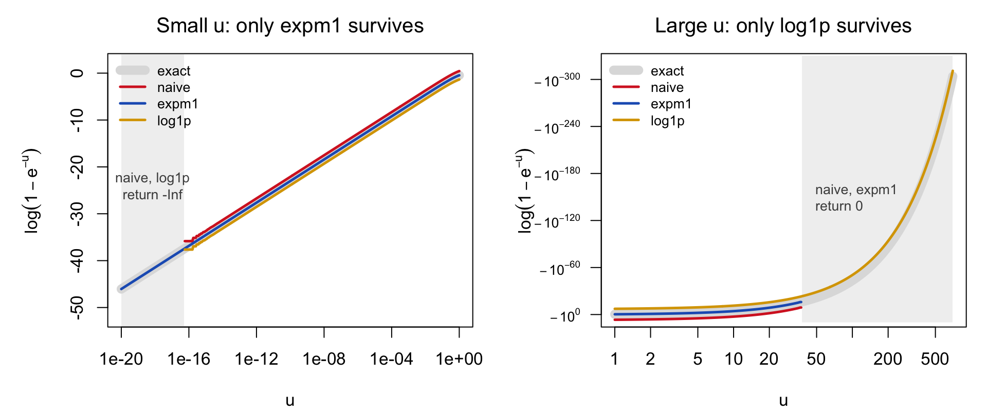
  • For small \(u\), naive tracks log1p: both lose digits and eventually collapse to \(-\infty\); only expm1 is correct.
  • For large \(u\), naive tracks expm1: both collapse to \(0\); only log1p is correct.
  • In the middle (\(10^{-8}\le u\le 20\)), all three agree, because \(u\) is nowhere near either landmark.

Solution: branch between the two remedies. Split at \(u=\log 2\), where \(e^{-u}=1/2\) is safely far from both traps, and use whichever incomplete remedy is valid on that side:

log1mexp <- function(u) ifelse(u <= log(2), log(-expm1(-u)), log1p(-exp(-u)))

The same construction, named log1mexp, is shipped by several CRAN packages (including copula and VGAM), all tracing to Mächler (2012); DPQ::logspace.sub(0, -u) computes the same quantity by an equivalent route. Prefer a package function in production code, and write your own only to understand why it works.

Figure 3.2 shows the three implementations against log1mexp (grey reference), on a log scale for \(u\): small \(u\) on the left, where only expm1 survives, and large \(u\) on the right, where only log1p survives.

fin <- function(y) replace(y, !is.finite(y), NA)   # -Inf: the curve simply stops
## for the right panel: place y < 0 on a log axis without changing its sign,
## by plotting log10(-y) against a reversed axis labelled -10^k
negpow <- function(y) {
  out <- rep(NA_real_, length(y)); ok <- is.finite(y) & y < 0
  out[ok] <- log10(-y[ok]); out
}
cols <- c(naive = "#D62728", expm1 = "#1F5FBF", log1p = "#D9A400")
par(mfrow = c(1, 2), mar = c(4.2, 5.2, 2.6, 1), cex = 1.05)

## left: small u, value plotted directly; jitter in units of the response
u <- 10^seq(-20, 0, length.out = 400)
jit <- c(0.9, 0, -0.9)
plot(u, log1mexp(u), type = "n", log = "x", ylim = c(-52, 2),
     xlab = expression(u), ylab = expression(log(1 - e^-u)),
     main = expression("Small" ~ u * ": only expm1 survives"))
u_dead <- max(u[!is.finite(f_naive(u))])
rect(min(u), -60, u_dead, 10, col = adjustcolor("gray50", 0.12), border = NA)
text(sqrt(min(u) * u_dead), -24, "naive, log1p\nreturn -Inf", col = "gray30", cex = 0.8)
lines(u, log1mexp(u), lwd = 9, col = "gray87")
lines(u, fin(f_naive(u)) + jit[1], lwd = 2.5, col = cols["naive"])
lines(u, fin(f_expm1(u)) + jit[2], lwd = 2.5, col = cols["expm1"])
lines(u, fin(f_log1p(u)) + jit[3], lwd = 2.5, col = cols["log1p"])
legend("topleft", bty = "n", cex = 0.8, lwd = c(9, 2.5, 2.5, 2.5),
       col = c("gray87", cols), legend = c("exact", "naive", "expm1", "log1p"))
## right: large u, same quantity on a log-magnitude axis (note the reversed ylim);
## jitter is now in powers of ten, so it must be applied after negpow()
u <- 10^seq(0, log10(700), length.out = 400)
jit <- c(7, 0, -7)
k <- seq(0, -300, by = -60)
plot(u, negpow(log1mexp(u)), type = "n", log = "x", ylim = c(3, -320), yaxt = "n",
     xlab = expression(u), ylab = expression(log(1 - e^-u)),
     main = expression("Large" ~ u * ": only log1p survives"))
axis(2, at = k, labels = parse(text = paste0("-10^", k)), las = 1, cex.axis = 0.8)
u_dead <- min(u[f_naive(u) >= 0])
rect(u_dead, 10, max(u), -330, col = adjustcolor("gray50", 0.12), border = NA)
text(u_dead * 1.3, -150, "naive, expm1\nreturn 0", adj = c(0, 0.5), col = "gray30", cex = 0.8)
lines(u, negpow(log1mexp(u)), lwd = 9, col = "gray87")
lines(u, negpow(f_naive(u)) + jit[1], lwd = 2.5, col = cols["naive"])
lines(u, negpow(f_expm1(u)) + jit[2], lwd = 2.5, col = cols["expm1"])
lines(u, negpow(f_log1p(u)) + jit[3], lwd = 2.5, col = cols["log1p"])
legend("topleft", bty = "n", cex = 0.8, lwd = c(9, 2.5, 2.5, 2.5),
       col = c("gray87", cols), legend = c("exact", "naive", "expm1", "log1p"))
Figure 3.2: Compares implementations of log(1 - exp(-u)) to show which formulas remain accurate for very small and very large u. The three implementations of log(1 - exp(-u)) against u on a log scale. Curves are offset vertically by a small constant so that they remain distinguishable where they agree; log1mexp is the grey reference.

3.3 Methods for Mitigating Overflow and Underflow Errors

3.3.1 Where overflow and underflow arise in statistics

Likelihoods are products of many probabilities, and normalizing constants involve factorials or exponentials: \[ \prod_{i=1}^{2000} p(x_i) = \left(\tfrac12\right)^{2000} \approx 10^{-602} \quad\to\quad \text{underflow to } 0, \] \[ 1000! \approx 4\times10^{2567} \quad\to\quad \text{overflow to } \infty, \] \[ \text{logistic: } \frac{e^{x}}{1+e^{x}} \text{ at } x = 1000 \quad\to\quad \frac{\infty}{\infty} = \texttt{NaN}. \]

Two remedies are available: change the algebraic expression so that the intermediate quantities stay in range, or work on the logarithmic scale.

3.3.2 Changing the algebraic expression

Two equivalent forms of the logistic (sigmoid) function: \[ \sigma(x) = \frac{e^{x}}{1+e^{x}} = \frac{1}{1+e^{-x}}. \]

\(x\) \(e^{x}/(1+e^{x})\) \(1/(1+e^{-x})\)
\(+1000\) \(e^{x}=\infty\), $/= $ NaN ✗ \(e^{-x}=0\), \(1/1 = 1\) ✓
\(-1000\) \(e^{x}=0\), \(0/1 = 0\) ✓ \(e^{-x}=\infty\), \(1/\infty = 0\) ✓

Evaluating the first form at a large positive value yields \(\infty/\infty\); the second form lets \(e^{-x}\) underflow harmlessly to \(0\) and computes \(1/(1+0) = 1\). In this case the second form is safe at both ends, because a division by \(\infty\) gives \(0\) correctly. In general one picks the form in which the exponential has a non-positive argument: \[ \sigma(x) = \begin{cases} 1/(1+e^{-x}) & x \ge 0\\ e^{x}/(1+e^{x}) & x < 0.\end{cases} \]

p1 <- function(theta) exp(theta) / (1 + exp(theta))
p2 <- function(theta) 1 / (1 + exp(-theta))

## large positive theta breaks p1, works in p2
theta <- 2000
c(p1 = p1(theta), p2 = p2(theta))
 p1  p2 
NaN   1 
## large negative theta works for both
theta <- -2000
c(p1 = p1(theta), p2 = p2(theta))
p1 p2 
 0  0 
## the piecewise form is safe everywhere and keeps full precision in both tails
sigmoid <- function(x) ifelse(x >= 0, 1 / (1 + exp(-x)), exp(x) / (1 + exp(x)))
sigmoid(c(-2000, -20, 0, 20, 2000))
[1] 0.000000000000000000000e+00 2.061153618190203325213e-09
[3] 5.000000000000000000000e-01 9.999999979388463078323e-01
[5] 1.000000000000000000000e+00

Built-in functions. Software provides functions written specifically to avoid cancellation and overflow, and they should be used in preference to the naive composition:

instead of use reason
log(1 + x) log1p(x) for tiny \(x\), 1 + x rounds to 1
exp(x) - 1 expm1(x) for tiny \(x\), exp(x) rounds to 1
log(factorial(n)) lfactorial(n), lgamma(n + 1) factorial(n) overflows
log(choose(n, k)) lchoose(n, k) overflow
log(dnorm(x)) dnorm(x, log = TRUE) dnorm(x) underflows
log(pnorm(x)) pnorm(x, log.p = TRUE) underflow
log(1 - pnorm(x)) pnorm(x, lower.tail = FALSE, log.p = TRUE) cancellation and underflow
c(naive = log(factorial(1000)), lfactorial = lfactorial(1000))
                  naive              lfactorial 
                    Inf 5912.128178488163939619 
c(naive = log(dnorm(40)), dnorm_log = dnorm(40, log = TRUE))
                   naive                dnorm_log 
                    -Inf -800.9189385332047095289 
c(naive = log(1 - pnorm(10)), stable = pnorm(10, lower.tail = FALSE, log.p = TRUE))
                   naive                   stable 
                    -Inf -53.23128515051246978373 

The last line shows both failures at once: 1 - pnorm(10) is 1 - 1 = 0 in double precision, so the naive answer is -Inf, while the true value is about \(-53.2\).

3.3.3 Representing numbers in logarithmic form

Represent a positive number \(x\) by \(\ell_x = \log x\): \[ x = e^{2000} \iff \ell_x = 2000, \qquad x = e^{-2000} \iff \ell_x = -2000 . \] Numbers that overflow or underflow in ordinary form are ordinary numbers on the log scale. The cost is that each operation \(f\) must be translated to the log scale: \[ x_1,\dots,x_n \xrightarrow{\;f\;} y \qquad\Longleftrightarrow\qquad \ell_1,\dots,\ell_n \xrightarrow{\;\tilde f\;} \ell_y = \log f(e^{\ell_1},\dots,e^{\ell_n}). \]

Products and quotients are the easy case: \[ \log(x_1 x_2) = \ell_1 + \ell_2, \qquad \log\left(\prod_{i=1}^{n} x_i\right) = \sum_{i=1}^{n} \ell_i, \qquad \log\frac{x_1}{x_2} = \ell_1 - \ell_2. \] In particular \(\log \prod_i p(x_i) = \sum_i \log p(x_i)\): always compute the log-likelihood, never the likelihood.

log_x <- 800; x <- exp(log_x); x          # overflow
[1] Inf
log_y <- 805; y <- exp(log_y); y          # overflow
[1] Inf
x / y                                     # Inf/Inf = NaN
[1] NaN
log_xovery <- log_x - log_y               # subtracting logs is safe
log_xovery
[1] -5
exp(log_xovery)
[1] 0.006737946999085467000845
## likelihood versus log-likelihood for 2000 fair-coin tosses
p <- rep(0.5, 2000)
c(likelihood = prod(p), log_likelihood = sum(log(p)))
             likelihood          log_likelihood 
    0.00000000000000000 -1386.29436111982249713 

3.3.4 The log-sum-exp trick

Sums are the hard case: \(\log(x_1 + x_2) \neq \ell_1 + \ell_2\). We need \[ \log\left(\sum_{i=1}^{n} x_i\right) = \log\left(\sum_{i=1}^{n} e^{\ell_i}\right), \] but the \(e^{\ell_i}\) may overflow or underflow. Let \(m = \max_i \ell_i\) and factor it out: \[ \log\left(\sum_{i=1}^{n} e^{\ell_i}\right) = \log\left(e^{m}\sum_{i=1}^{n} e^{\ell_i - m}\right) = m + \log\left(\sum_{i=1}^{n} e^{\ell_i - m}\right). \]

Every \(\ell_i - m \le 0\), so \(e^{\ell_i - m} \in (0, 1]\) and nothing overflows; the largest term is \(e^{0} = 1\), so the sum is at least 1 and cannot underflow. Terms far below the maximum underflow to \(0\) individually, but they would have contributed nothing at 16-digit precision anyway.

Illustration with \(x_i = e^{2000}, e^{2001}, e^{2002}\), each of which overflows to Inf:

\(i=1\) \(i=2\) \(i=3\)
\(\ell_i\) 2000 2001 2002
\(\ell_i - m\) (\(m = 2002\)) \(-2\) \(-1\) \(0\)
\(e^{\ell_i - m}\) \(0.135\) \(0.368\) \(1\)

\[ \log\sum_i x_i = 2002 + \log(0.135 + 0.368 + 1) = 2002.408 \]

log_sum_exp <- function(log_x) {
  max_log_x <- max(log_x)
  max_log_x + log(sum(exp(log_x - max_log_x)))
}

## values that would overflow directly
log_x <- c(2000, 2010, 2030)
exp(log_x)                                   # Inf
[1] Inf Inf Inf
c(direct = log(sum(exp(log_x))), lse = log_sum_exp(log_x))
                 direct                     lse 
                    Inf 2030.000000002061142368 
## values that would underflow directly
log_x <- -c(2000, 2010, 2030)
exp(log_x)                                   # 0
[1] 0 0 0
c(direct = log(sum(exp(log_x))), lse = log_sum_exp(log_x))
                 direct                     lse 
                   -Inf -1999.99995460110062595 

Example: log-likelihood of a mixture. The density of a two-component normal mixture is \(f(y) = \pi_1\varphi(y;\mu_1,1) + \pi_2\varphi(y;\mu_2,1)\), a sum inside a product. For an observation far from both means, both component densities underflow and the naive log-likelihood is -Inf; with log-sum-exp applied observation by observation it is finite and correct.

y <- c(-1, 0.5, 2, 45)                      # the last value is far from both means
mu <- c(0, 3); w <- c(0.6, 0.4)
naive <- sum(log(w[1] * dnorm(y, mu[1]) + w[2] * dnorm(y, mu[2])))
stable <- sum(sapply(y, function(yi) log_sum_exp(log(w) + dnorm(yi, mu, log = TRUE))))
c(naive = naive, stable = stable)
                   naive                   stable 
                    -Inf -889.3332627696936469874 

Example: log-softmax. The softmax probabilities \(p_k = e^{x_k}/\sum_j e^{x_j}\) appear in multinomial logistic regression and neural networks. Their logarithm is \(\log p_k = x_k - \log\sum_j e^{x_j}\), and the second term is a log-sum-exp.

x <- c(1000, 1001, 1005)
naive <- log(exp(x) / sum(exp(x)))
stable <- x - log_sum_exp(x)
rbind(naive, stable, probabilities = exp(stable))
                                     [,1]                      [,2]
naive                                 NaN                       NaN
stable        -5.024744890138777009269688 -4.0247448901387770092697
probabilities  0.006573263185309382618249  0.0178679818703053189255
                                    [,3]
naive                                NaN
stable        -0.02474489013877700926969
probabilities  0.97555875494443089479546

Software implementation. The log-sum-exp trick is already implemented, tested, and optimized in the matrixStats package (a dependency of hundreds of CRAN/Bioconductor packages), so production code should call it rather than the version above:

library(matrixStats)
c(mine = log_sum_exp(c(2000, 2001, 2002)), matrixStats = logSumExp(c(2000, 2001, 2002)))
                   mine             matrixStats 
2002.407605964444428537 2002.407605964444428537 

3.3.5 Differences on the log scale

For \(x > y > 0\) with \(\ell_x = \log x\), \(\ell_y = \log y\): \[ \log(x - y) = \log\left(e^{\ell_x}\left(1 - e^{\ell_y - \ell_x}\right)\right) = \ell_x + \log\left(1 - e^{\ell_y - \ell_x}\right). \] Since \(\ell_y - \ell_x < 0\), \(e^{\ell_y-\ell_x}\in(0,1)\) and there is no overflow. When \(x \approx y\), the factor \(1 - e^{\ell_y-\ell_x}\) is itself a large − large subtraction; log1p(-exp(ly - lx)) avoids it.

log_minus_exp <- function(log_x, log_y) {
  if (log_x < log_y) stop("the first argument must be the larger")
  log_x + log1p(-exp(log_y - log_x))
}

log_minus_exp(2020, 2000)
[1] 2019.999999997938857632
exp(2000) - exp(1999)                       # direct subtraction: Inf - Inf = NaN
[1] NaN
## nearly equal arguments: log1p keeps the precision that log(1 - .) would lose
lx <- 10; ly <- 10 - 1e-12
c(with_log1p = log_minus_exp(lx, ly), with_log = lx + log(1 - exp(ly - lx)), exact = log(exp(lx) - exp(ly)))
              with_log1p                 with_log                    exact 
-17.63093221929763032563 -17.63093221929763032563 -17.63078806616063687329 

A statistical use of the difference formula is the survival function of a discrete distribution, \(\log P(X > k) = \log\big(1 - P(X\le k)\big)\), when \(P(X\le k)\) is available only as a log-probability close to \(0\).

Four extreme choices of \(a,b\) show that every one of the four failure modes met in this chapter — overflow, cancellation, underflow, and absorption — can destroy a naive log(exp(a) - exp(b)), and that log_minus_exp survives all four because it never forms exp(a) or exp(b) when they would be out of range:

a <- c(2000, 1e-20, -1000,    0)
b <- c(1999,     0, -1001, -500)
g <- function(x) formatC(x, format = "g", digits = 8)
kable(data.frame(a = g(a), b = g(b), u = g(a - b),
                  naive = g(log(exp(a) - exp(b))),
                  log_minus_exp = g(mapply(log_minus_exp, a, b))),
      caption = "Shows why log(exp(a) - exp(b)) should be computed on the log scale: the naive expression overflows for large a and b, whereas log_minus_exp stays finite and accurate. log(exp(a) - exp(b)) by the naive expression and by log_minus_exp",
      align = c("r", "r", "r", "r", "r"))
Shows why log(exp(a) - exp(b)) should be computed on the log scale: the naive expression overflows for large a and b, whereas log_minus_exp stays finite and accurate. log(exp(a) - exp(b)) by the naive expression and by log_minus_exp
a b u naive log_minus_exp
2000 1999 1 NaN 1999.5413
1e-20 0 1e-20 -Inf -Inf
-1000 -1001 1 -Inf -1000.4587
0 -500 500 0 -7.1245764e-218

Reading down the naive column: \(\log(e^{2000}-e^{1999})\) is Inf - Inf, NaN (overflow); \(\log(e^{10^{-20}}-e^{0})\) is 1 - 1, so \(-\infty\) (cancellation, since \(u=10^{-20}\) is tiny); \(\log(e^{-1000}-e^{-1001})\) is 0 - 0, so \(-\infty\) (underflow, even though \(u=1\) is not small); and \(\log(e^{0}-e^{-500})\) silently returns \(0\) because \(e^{-500}\approx7\times10^{-218}\) is absorbed into \(1\) before the subtraction (absorption). log_minus_exp is correct in all four rows, because it factors out \(e^{a}\) and reduces every case to log1p evaluated at a safely bounded argument — even recovering the tiny but nonzero last entry. The same function is available as DPQ::logspace.sub, with DPQ::logspace.add as the corresponding stable version of \(\log(e^{a}+e^{b})\) for a single pair (logSumExp above is the version for a whole vector).

3.3.6 A combined example: \(\log\{1-\Phi(x)\}\) at both tails

The rounding fix log1mexp, developed earlier for \(\log(1-e^{-u})\), and the underflow fix of working on the log scale are often needed together. Consider \(\log\{1-\Phi(10)\}\) and \(\log\{1-\Phi(-10)\}\), where \(\Phi\) is the standard normal CDF (pnorm):

c(naive    = log(1 - pnorm(10)),                          # pnorm(10) rounds to 1, so log(0) = -Inf
  log1p    = log1p(-pnorm(10)),                            # log1p cannot recover digits already lost
  log1mexp = log1mexp(-pnorm(10, log.p = TRUE)),           # complement taken in log space
  stable   = pnorm(10, lower.tail = FALSE, log.p = TRUE))  # direct upper tail
                   naive                    log1p                 log1mexp 
                    -Inf                     -Inf -53.23128515051246978373 
                  stable 
-53.23128515051246978373 

The target is \(\log\{1-\Phi(10)\}\approx-53.23\), since \(1-\Phi(10)\approx7.6\times10^{-24}\) is far below machine epsilon. naive and log1p both start from pnorm(10), which has already rounded to exactly \(1\) before either function is called, so no reformulation of the outer expression can recover digits lost by underflow inside pnorm itself. log1mexp instead starts from \(\ell=\log\Phi(10)\approx-7.6\times10^{-24}\), which R returns accurately, and computes \[ \log\{1-\Phi(10)\} = \log(1-e^{\ell}) = \log(1-e^{-u}) = \texttt{log1mexp}(u), \qquad u=-\ell, \] where the tiny \(u\) correctly selects the expm1 branch derived above. stable computes \(1-\Phi(10)\) directly with lower.tail = FALSE and returns its log without ever forming \(\Phi(10)\).

c(naive    = log(1 - pnorm(-10)),                           # 1 - 7.6e-24 rounds to 1, so log gives 0
  log1p    = log1p(-pnorm(-10)),                             # pnorm(-10) is itself accurate
  log1mexp = log1mexp(-pnorm(-10, log.p = TRUE)),
  stable   = pnorm(-10, lower.tail = FALSE, log.p = TRUE))
                       naive                        log1p 
 0.000000000000000000000e+00 -7.619853024160526919908e-24 
                    log1mexp                       stable 
-7.619853024160532797379e-24 -7.619853024160526919908e-24 

Here \(\Phi(-10)\approx7.6\times10^{-24}\) and the target \(\log\{1-\Phi(-10)\}\approx-7.6\times10^{-24}\) is a tiny negative number rather than a large one. naive now fails for the opposite reason: the subtraction \(1-7.6\times10^{-24}\) itself rounds to exactly \(1\), destroying every significant digit — cancellation, not underflow. log1p succeeds here because its argument pnorm(-10) is accurate (a number near \(0\) keeps full relative precision) and log1p evaluates \(\log(1+x)\) by series without ever forming \(1+x\). log1mexp is again correct, but now via its log1p branch: \(\ell=\log\Phi(-10)\approx-53.23\), so \(u=-\ell=53.23\) is large.

The contrast between the two examples is the location of the loss: at \(x=10\) the damage occurs inside pnorm(10) before log1p is ever reached; at \(x=-10\) only the outer subtraction is unstable, which is exactly what log1p fixes. The general lesson is to stay on the log scale throughout — ask R for \(\log\Phi(x)\) rather than \(\Phi(x)\), and take the complement with log1mexp, which selects the correct branch automatically so that the tail direction never has to be diagnosed by hand.

3.4 Summary

  • Integers occupy a fixed number of bits; exceeding \(2^{31}-1\) gives NA in R.

  • Doubles store a sign, a 52-bit mantissa (about 16 decimal digits), and an 11-bit exponent (magnitudes \(10^{-308}\) to \(10^{308}\)). Neighbouring doubles are spaced at a relative distance of about \(\epsilon = 2^{-52}\); integers above \(2^{53}\) are not all representable.

  • Overflow produces Inf, underflow produces 0; the latter is silent and therefore more dangerous.

  • Roundoff error is amplified by adding large + small (fix: add small terms first, pairwise or compensated summation) and by subtracting large − large (fix: reformulate so that same-sign quantities of similar size are combined, as in \(e^{-x} = 1/e^{x}\) and the two-pass variance). Some quantities, such as \(\log(1-e^{-u})\), suffer from both failure modes at opposite ends of their range and need a function like log1mexp that branches between two incomplete remedies (expm1, log1p).

  • Overflow and underflow are avoided by rewriting expressions so that exponentials have non-positive arguments, by using purpose-built functions (log1p, expm1, lgamma, dnorm(log = TRUE)), and by working on the log scale, where products become sums and sums are handled by the log-sum-exp trick (log_sum_exp/matrixStats::logSumExp for a vector, log_minus_exp/DPQ::logspace.sub for a difference of two).

  • Rounding and underflow fixes often compose: computing \(\log\{1-\Phi(x)\}\) correctly at both tails needs pnorm(x, log.p = TRUE) to avoid underflow and log1mexp to avoid cancellation, in either order depending on the sign of \(x\).

3.5 Exercises

Question 1. How do you compute \[ \log\left(\frac{1}{1+e^{-x}}\right), \] so as to avoid overflow and underflow of \(e^{-x}\), for both large positive and large negative \(x\)? (Hint: write it as \(-\log(1+e^{-x})\) and consider log1p and the two forms of the sigmoid.)

Question 2 (log-softmax). How do you compute \[ \log\left(\frac{e^{x_k}}{\sum_{j=1}^{K} e^{x_j}}\right), \] so as to avoid underflow and overflow of \(e^{x_j}\)? Verify your formula against the log-softmax example above for \(x = (1000, 1001, 1005)\) and for \(x = (-1000, -1001, -1005)\).

Question 3. The one-pass variance formula fails for \(x = (M+1, M+2, M+3)\) with \(M = 10^{8}\). Predict the smallest \(M\) (a power of 10) at which the one-pass result in R first differs from \(2\), then verify using the scan in the variance section.

Question 4. Write a function log_dbinom(k, n, p) that returns \(\log\binom{n}{k}p^k(1-p)^{n-k}\) for \(n = 10^5\) without overflow or underflow, using lchoose and log1p, and compare it with dbinom(k, n, p, log = TRUE).

Question 5. Implement Welford’s algorithm for the sample covariance of two variables and check it against cov() on data shifted by \(10^{10}\).

Question 6. For a Poisson(\(\lambda\)) random variable, \(\log P(X > 0) = \log(1-e^{-\lambda})\). Using log1mexp, compute this for \(\lambda = 10^{-12}\) and for \(\lambda = 700\), and explain in each case which of expm1 or log1p alone would have failed and why.