The previous chapter approximated an integral by a weighted sum of function values on a grid. A grid gets expensive fast: an \(n\)-point-per-axis product grid costs \(n^d\) evaluations, so quadrature is only practical for \(d \lesssim
3\). The Laplace approximation takes a completely different route: instead of evaluating the integrand everywhere, it looks only at the single most important point — the mode — and replaces the whole integrand there by the Gaussian that matches its height and curvature. No grid is needed at any dimension, at the price of assuming the integrand is roughly bell-shaped.
9.1 The Goal and the Idea
Many Bayesian calculations are posterior expectations \[
E_f\big[a(\theta)\big] = \frac{\int a(\theta)\,f(\theta)\,d\theta}{\int f(\theta)\,d\theta},
\] where \(\theta \in \mathbb{R}^p\), \(a(\theta)\) is some quantity of interest (a parameter, a prediction, an indicator), and \(f(\theta)\) is an unnormalized posterior, typically \(f(\theta) = L(\theta)\pi(\theta)\). Both numerator and denominator are \(p\)-dimensional integrals.
Write \(h(\theta) = -\log f(\theta)\), so \(f(\theta) = e^{-h(\theta)}\). For independent data, \(h\) is (up to an additive constant) minus the log-likelihood plus minus the log-prior — a sum of \(n\) terms — so as \(n\) grows it becomes large and sharply curved at its minimum. This is the same large-sample regularity that makes the MLE asymptotically normal (seen in the maximum-likelihood chapters); here it makes the posterior asymptotically normal too. The Laplace approximation makes this precise by expanding \(h\) to second order at its minimum and integrating the resulting Gaussian exactly — no grid, no sampling, just one optimization and one Hessian.
9.2 Derivation
Let \(\theta_0 = \arg\min_\theta h(\theta)\), the posterior mode, found numerically (optim(..., hessian = TRUE) or nlm(..., hessian = TRUE) in R — exactly the optimizers used to find the MLE in earlier chapters). Expand \(h\) around \(\theta_0\): \[
h(\theta) = h(\theta_0) + \underbrace{\nabla h(\theta_0)^\top}_{=\,0\text{ at the minimum}}(\theta - \theta_0)
+ \tfrac12(\theta-\theta_0)^\top H (\theta - \theta_0) + O\big(\|\theta-\theta_0\|^3\big),
\qquad H = \nabla^2 h(\theta_0).
\]\(H\), the Hessian of \(-\log f\) at the mode, is positive definite at a genuine minimum; for \(f = L\pi\) it is the observed information plus the curvature of the log-prior. Dropping the cubic remainder and exponentiating, \[
f(\theta) \approx \tilde f(\theta) = f(\theta_0)\exp\Big\{-\tfrac12(\theta-\theta_0)^\top H(\theta-\theta_0)\Big\}
= \underbrace{f(\theta_0)(2\pi)^{p/2}|H|^{-1/2}}_{\text{constant}}
\cdot \underbrace{(2\pi)^{-p/2}|H|^{1/2}e^{-\frac12(\theta-\theta_0)^\top H(\theta-\theta_0)}}_{N_p(\theta_0,\,H^{-1})\text{ density}}.
\] Two results follow immediately, since the bracketed factor is a properly normalized \(N_p(\theta_0, H^{-1})\) density:
Only the mode and the Hessian of \(-\log f\) at the mode are needed — both come for free from any optimizer that returns a Hessian. The relative error of the second result is \(O(1/n)\) for regular models; the error of the first is governed by how skewed the true posterior actually is.
9.3 Worked Example: A Poisson Rate with a Gamma Prior
To see the approximation against ground truth, use a model with a known exact answer: the Gamma–Poisson conjugate pair from the Bayesian Inference chapter. For \(y_1,\ldots,y_n \mid \lambda \sim \text{Poisson}(\lambda)\) and \(\lambda \sim \text{Gamma}(\alpha,\beta)\), the posterior is exactly \(\text{Gamma}(\alpha + \sum y_i,\ \beta+n)\), and the marginal likelihood derived there in closed form, \(\log P(\mathbf y) = \alpha\log\beta - \log\Gamma(\alpha) + \log\Gamma(\alpha+S)
- (\alpha+S)\log(\beta+n) - \sum_i\log(y_i!)\) with \(S=\sum_i y_i\), is exactly exact_log_ml below — so both the exact log marginal likelihood and the exact posterior are available to measure the Laplace error directly.
Code
alpha <-2; beta <-1### Laplace approximation: mode, Hessian, and the two boxed results abovelaplace_poisson <-function(y) { h <-function(l) -(sum(dpois(y, l, log =TRUE)) +dgamma(l, alpha, beta, log =TRUE)) op <-optim(mean(y) +0.5, h, method ="L-BFGS-B", lower =1e-6, hessian =TRUE)c(mode = op$par, se =sqrt(1/ op$hessian[1, 1]),log_ml =-op$value +0.5*log(2* pi) -0.5*log(op$hessian[1, 1]))}### exact log marginal likelihood, from the Gamma-Poisson conjugate identityexact_log_ml <-function(y) { n <-length(y); s <-sum(y) alpha *log(beta) -lgamma(alpha) +lgamma(alpha + s) - (alpha + s) *log(beta + n) -sum(lfactorial(y))}
Table 9.1: Assesses the accuracy of the Laplace approximation by comparing it with the exact marginal likelihood in a conjugate example where the exact answer is known. Laplace log marginal likelihood versus the exact value, and the posterior mean versus the Laplace mode, as n grows. The error shrinks roughly like 1/n: it falls by about a factor of 4-5 each time n increases by that factor.
n
Laplace log P(y)
exact log P(y)
error
Laplace mode
posterior mean
5
-11.3822
-11.3784
-0.0038
3.6667
3.8333
20
-44.2274
-44.2263
-0.0011
3.6190
3.6667
100
-197.0022
-197.0019
-0.0003
2.9406
2.9505
500
-958.5983
-958.5983
-0.0001
2.8842
2.8862
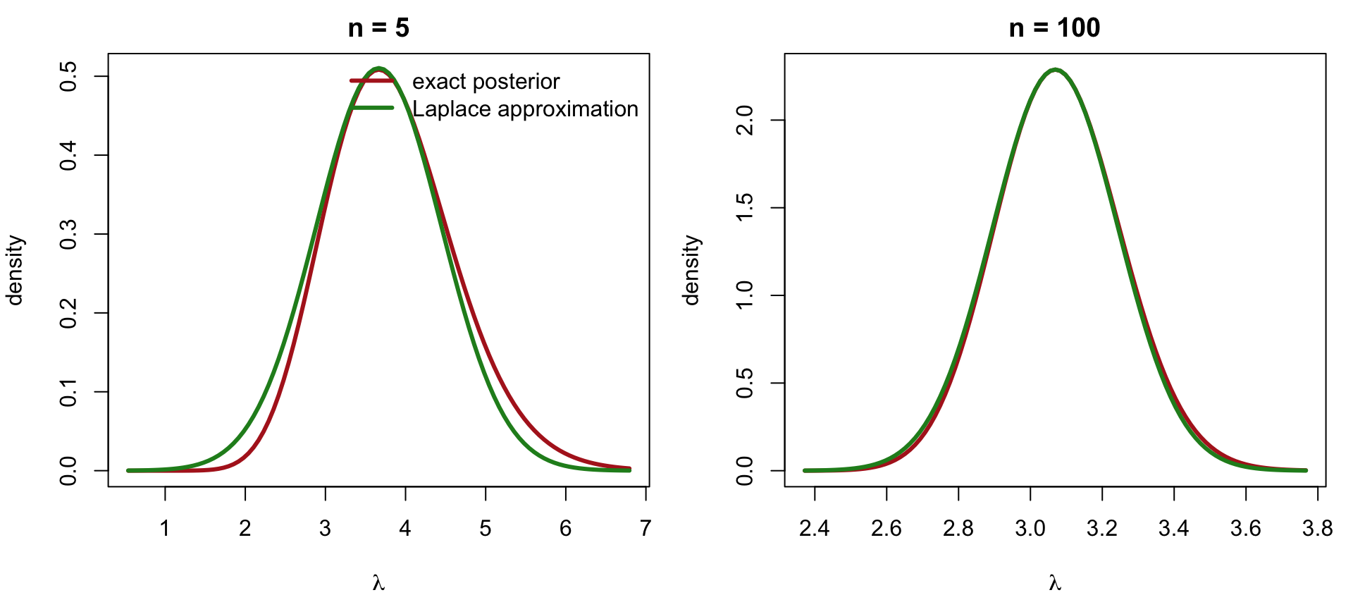
The error is a few thousandths at \(n=5\) and shrinks to a few ten-thousandths by \(n=500\); the Laplace mode also converges to the posterior mean as the Gamma posterior becomes more symmetric. Plotting the exact posterior against its Laplace approximation makes this concrete:
Code
par(mfrow =c(1, 2), mar =c(4, 4, 2, 1))set.seed(42)for (n inc(5, 100)) { y <-rpois(n, 3); a1 <- alpha +sum(y); b1 <- beta + n lap <-laplace_poisson(y)curve(dgamma(x, a1, b1), max(0, lap["mode"] -4* lap["se"]), lap["mode"] +4* lap["se"],lwd =3, col ="firebrick", xlab =expression(lambda), ylab ="density",main =sprintf("n = %d", n))curve(dnorm(x, lap["mode"], lap["se"]), add =TRUE, lwd =3, col ="forestgreen")if (n ==5) legend("topright", bty ="n", lwd =3, col =c("firebrick", "forestgreen"),legend =c("exact posterior", "Laplace approximation"))}
Figure 9.1: Shows how the Laplace approximation replaces a posterior by a normal density centred at the mode, and how well it fits at small and large sample sizes. Exact Gamma posterior (red) and the Laplace normal approximation (green) for n=5 and n=100. At n=5 the exact posterior is visibly right-skewed and the Gaussian is a rough match; by n=100 the two are nearly indistinguishable, illustrating the O(1/n) convergence in the table above.
9.3.1 Linear functionals: posterior mean and credible intervals
If \(a(\theta) = A^\top\theta + a_0\) is linear, replacing \(f\) by \(\tilde f\) gives \(E_f[a(\theta)] \approx A^\top\theta_0 + a_0\): the posterior mean is approximated by the posterior mode, and \(\text{Var}(A^\top\theta) \approx
A^\top H^{-1}A\) gives Wald-style credible intervals \(\theta_{0j} \pm
z_{\alpha/2}\sqrt{(H^{-1})_{jj}}\) — exactly the Bayesian counterpart of an MLE plus its Wald standard error from the maximum-likelihood chapters.
Table 9.2: Compares interval estimates based on the Laplace approximation with the exact posterior intervals, to see how much accuracy is lost. Laplace mode/SE-based 95% interval versus the exact Gamma posterior mean/sd-based interval, n = 20.
quantity
center
spread
lower95
upper95
mode
Laplace (mode / se)
3.6190
0.4151
2.8054
4.4327
exact posterior (mean / sd)
3.6667
0.4179
2.8937
4.5298
The two intervals agree closely even at \(n=20\): the mild right-skew of the Gamma posterior visible in Figure 9.1 has not yet noticeably distorted a Wald-style interval built from a symmetric Gaussian.
9.3.2 BIC as a large-\(n\) simplification
With \(f(\theta) = L(\theta;D)\pi(\theta)\), the Laplace approximation to the log marginal likelihood is \[
\log P(D) \approx \log\big[L(\theta_0;D)\,\pi(\theta_0)\big] + \frac p2\log(2\pi) - \frac12\log|H|.
\] For large \(n\) the Hessian is dominated by the likelihood, \(H \approx
n\,I(\theta_0)\) with \(I\) the per-observation Fisher information, so \(|H|
\approx n^p|I(\theta_0)|\) and \[
\log P(D) \approx \log L(\theta_0;D) - \frac p2\log n
+ \underbrace{\log\pi(\theta_0) + \frac p2\log(2\pi) - \frac12\log|I(\theta_0)|}_{O(1),\text{ dropped}}.
\] Multiplying by \(-2\) and replacing the posterior mode by the MLE (the two coincide to \(O(1/n)\)) gives the Bayesian information criterion, \(\text{BIC} = -2\log L(\hat\theta_{\text{MLE}}) + p\log n\) — a model-comparison score that needs no prior at all, because the dropped \(O(1)\) terms do not grow with \(n\) and so wash out of differences between models fit to the same data. For the \(n=20\) Poisson example from the credible-interval check above, \(-2\times(\text{Laplace log }P(y))\) and the MLE-based BIC differ by about 1.68 — a constant offset consistent with the dropped \(O(1)\) terms, not something that grows with \(n\).
9.3.3 When Laplace Works Well, and When It Does Not
Works well when \(n\) is large relative to \(p\) and the posterior is unimodal and roughly symmetric, as in the \(n=100\) panel above. Parameters should live on an unbounded scale — transform first (\(\log\sigma\), \(\text{logit}\,p\)) so the matching Gaussian is not truncated at a boundary, remembering to include the Jacobian of the transform in \(f\) (exactly the \(w=\log\sigma^2\) reparametrization used throughout this book since the multivariate optimization chapter).
Struggles when the posterior is skewed (small \(n\), a parameter near a boundary) — the mode is then a poor stand-in for the mean and the Gaussian tails are wrong, as the \(n=5\) panel above already shows mildly; when the posterior is multimodal, since the approximation only sees the one mode an optimizer happened to find; and in hierarchical models where \(p\) grows with \(n\), so the \(O(1/n)\) error does not vanish (nested Laplace approximation, INLA, handles this by integrating out the high-dimensional part analytically).
9.4 Example: Comparing Laplace, Quadrature, and Monte Carlo on Computing Marginal Likelihood
To compare the three methods on an apples-to-apples problem, reuse the single-parameter example from the end of Unit 08: a single unknown mean \(\mu\), with likelihood \[
L(\mu) = N\big(\hat\mu;\,\mu,\,1/n_{\text{eff}}\big),
\] treating \(\hat\mu\) as the sample mean of \(n_{\text{eff}}\) observations from \(N(\mu,1)\), under a prior \(\pi(\mu) = N(\mu;0,5^2)\). The marginal likelihood is \[
P(y) = \int_{-\infty}^{\infty} z(\mu)\,d\mu, \qquad z(\mu) = \pi(\mu)L(\mu).
\] Because this is a normal-normal conjugate pair, \(P(y)\) has a closed form, so a genuine true value is available for comparison — computed here by numerical integration, exactly as in Unit08, rather than by writing out the closed-form expression. Laplace attacks the integral by optimization instead of a grid: find the mode of \(z(\mu)\) and the second derivative of \(-\log z\) there, then apply the boxed formula with \(p=1\). Quadrature attacks it with the logistic-transform midpoint rule from Unit08. Monte Carlo with \(\pi\) attacks it by drawing \(\mu\) directly from the prior and averaging the likelihood — the same naive estimator used throughout Unit08.
Code
n_eff <-3; sigma_prior <-5# same setup as the Unit08 app### true value: exact up to numerical-integration error, since z is a### normal-normal conjugate kernellog_mar_true_mu <-function(mu_hat) { z <-function(mu) dnorm(mu_hat, mu, 1/sqrt(n_eff)) *dnorm(mu, 0, sigma_prior)log(integrate(z, -Inf, Inf)$value)}### Laplace: p = 1 case of the boxed formula, mode and Hessian from nlm()laplace_mu <-function(mu_hat) { h <-function(mu) -(dnorm(mu_hat, mu, 1/sqrt(n_eff), log =TRUE) +dnorm(mu, 0, sigma_prior, log =TRUE)) op <-nlm(h, p = mu_hat, hessian =TRUE)c(mode = op$estimate, log_ml =-op$minimum +0.5*log(2* pi) -0.5*log(op$hessian[1, 1]))}### naive Monte Carlo: draw mu from the prior, average the likelihoodlog_sum_exp <-function(lx) { m <-max(lx); m +log(sum(exp(lx - m))) }log_mar_mc_mu <-function(mu_hat, iters) { mus <-rnorm(iters, 0, sigma_prior)log_sum_exp(dnorm(mu_hat, mus, 1/sqrt(n_eff), log =TRUE)) -log(iters)}### midpoint rule on the logistic-transformed (0, 1) grid, as in Unit08log_mar_mid_mu <-function(mu_hat, n) { h <-1/ n u <- (seq_len(n) -0.5) * h mu <-log(u / (1- u)) log_z <-dnorm(mu_hat, mu, 1/sqrt(n_eff), log =TRUE) +dnorm(mu, 0, sigma_prior, log =TRUE) -log(u * (1- u))log_sum_exp(log_z) +log(h)}
Table 9.3: Compares the Laplace approximation with grid quadrature and naive Monte Carlo against the true value as the posterior moves away from the prior mean, to show where each method succeeds or fails. Log marginal likelihood by four methods, for data locations mu_hat = 0, -5, -20 (n_eff = 3, sigma = 1, prior N(0, 5^2) on mu). Quadrature uses a 100-point midpoint grid; Monte Carlo uses 1e6 prior draws; both are unchanged from Unit08’s app.
mu
True
Laplace
Monte Carlo (pi)
Quadrature (n=100)
0
-2.535
-2.535
-2.537
-2.535
-5
-3.028
-3.028
-3.027
-2.707
-20
-50.734
-10.430
-10.626
-327.191
At \(\mu=0\) the posterior sits right where both the logistic grid and the prior put their effort, so all four numbers should agree closely. As \(\mu\) moves to \(-5\) and then \(-20\), the fixed grid — centred at \(0\) by construction — squeezes the posterior into an ever-thinner sliver of the unit interval, and quadrature is the first to break away from the true value, exactly the failure diagnosed at the end of Unit08. Naive Monte Carlo is built on the same fragile assumption in a different guise: it needs prior draws near\(\mu\) to contribute any likelihood at all, so once \(\mu\) is several prior standard deviations from \(0\), a fixed budget of draws from \(\pi\) can also become too sparse there to be trusted, even though nothing about the Monte Carlo estimator’s derivation assumed \(\mu\) would be small. Laplace has neither failure mode: it optimizes to find the mode wherever it actually is and builds its approximation around that point, so it automatically “recentres” itself for every \(\mu\) — the same fix Unit08 proposed by hand for quadrature, done here for free by the optimizer.
9.5 Adaptive Gauss–Hermite Quadrature
A fixed logistic transform (\(u=1/(1+e^{-\mu})\)) fails when the posterior mass moves far from \(\mu=0\). Adaptive Gauss-Hermite quadrature (AGHQ) solves this by relocating and rescaling the quadrature grid using the Laplace approximation’s mode (\(\hat\mu_L\)) and standard deviation (\(s_L=1/\sqrt{H}\)).
Think of it as a smart, localized search grid: instead of laying a massive grid over the entire parameter space, AGHQ finds the peak of the posterior (the mode), measures its exact curvature (the Hessian), and places a custom-scaled grid directly over that localized area.
By swapping the logistic function for the CDF and density of \(N(\hat\mu_L, s_L^2)\), the transform becomes: \[
u = \Phi\!\left(\frac{\mu-\hat\mu_L}{s_L}\right), \qquad \mu = \hat\mu_L + s_L\,\Phi^{-1}(u), \qquad \frac{du}{d\mu} = \phi\!\left(\frac{\mu-\hat\mu_L}{s_L}\right)
\]
Applying a midpoint rule on this adapted grid yields: \[
P(y) \approx \frac1n\sum_{i=1}^n \frac{z(\mu_i)}{\phi\big((\mu_i-\hat\mu_L)/s_L\big)/s_L}, \qquad \mu_i = \hat\mu_L + s_L\,\Phi^{-1}(u_i), \qquad u_i = \big(i-\tfrac12\big)/n
\]
9.5.1 Shinylive App for Adaptive Gauss–Hermite Quadrature
There is a shinylive app to show how centring and scaling the quadrature grid with the Laplace approximation lets a few grid points capture the posterior wherever it sits.
9.6 Summary
The Laplace approximation expands \(h=-\log f\) to second order at its minimum \(\theta_0\) and integrates the resulting Gaussian exactly: \(\theta\mid\text{data} \approx N_p(\theta_0, H^{-1})\) and \(\int f(\theta)\,d\theta \approx f(\theta_0)(2\pi)^{p/2}|H|^{-1/2}\).
It needs only an optimizer and a Hessian — the same machinery already used to find the MLE — and its cost does not grow with dimension the way a quadrature grid’s does.
BIC is the large-\(n\) simplification of the Laplace marginal likelihood, dropping \(O(1)\) terms that do not depend on the sample size.
On the running Gaussian marginal-likelihood example, Laplace tracked the true value everywhere it was tested, including where quadrature’s fixed grid broke down and even where naive Monte Carlo’s fixed proposal started to run short of relevant draws — because Laplace re-optimizes for every dataset instead of committing to one grid or one proposal in advance.
It is deterministic, fast, and accurate to \(O(1/n)\), but blind to skewness and multimodality; the Monte Carlo methods of the next chapters remove these limitations at higher computational cost.