2 Data Science with R and Quarto

Author

Affiliation

University of Saskatchewan

Published

November 26, 2025

2.1 Basic R Objects and Operations

Code

## create a vector
x <- 1:10
x <- seq (30,3, by = -2)
a <- c(66.32, 69.87, 70.12, 90.37, 50.08, 61.20, 65.00, 57.65)
d <- a [1]
a [1] <- 85.34

mean (a)

[1] 68.70375

Code

ma <- mean (a)
## read a vector of numbers from a file
x <- scan("numbers.txt")
x2 <- scan("number2.txt")

## one can also read number withoug saving to a file
y <- scan(text = "7  8  9 10 11 12 13 13 14 17 17 45")

## create a matrix
A <- matrix (0, 4, 2)

A <- matrix (1:8, 4,2)

A

     [,1] [,2]
[1,]    1    5
[2,]    2    6
[3,]    3    7
[4,]    4    8

Code

D <- matrix (a, 4, 2, byrow=T)

D <- matrix(1:8, 2, 4)
D

     [,1] [,2] [,3] [,4]
[1,]    1    3    5    7
[2,]    2    4    6    8

Code

## create another matrix with all entry 0
B <- matrix (1:5000, 100, 50)

## assign a number to B
B[2,4] <- 45
B[1,]

 [1]    1  101  201  301  401  501  601  701  801  901 1001 1101 1201 1301 1401
[16] 1501 1601 1701 1801 1901 2001 2101 2201 2301 2401 2501 2601 2701 2801 2901
[31] 3001 3101 3201 3301 3401 3501 3601 3701 3801 3901 4001 4101 4201 4301 4401
[46] 4501 4601 4701 4801 4901

Code

B[,1]

  [1]   1   2   3   4   5   6   7   8   9  10  11  12  13  14  15  16  17  18
 [19]  19  20  21  22  23  24  25  26  27  28  29  30  31  32  33  34  35  36
 [37]  37  38  39  40  41  42  43  44  45  46  47  48  49  50  51  52  53  54
 [55]  55  56  57  58  59  60  61  62  63  64  65  66  67  68  69  70  71  72
 [73]  73  74  75  76  77  78  79  80  81  82  83  84  85  86  87  88  89  90
 [91]  91  92  93  94  95  96  97  98  99 100

Code

B[1,] <- 1:50


## create a list
E <- list (newa = a, newA = A)
## list the names of components
names (E)

[1] "newa" "newA"

Code

## to look at the component of E
E$newA

     [,1] [,2]
[1,]    1    5
[2,]    2    6
[3,]    3    7
[4,]    4    8

Code

E$newa <- 10:17

## create a dataframe
scores <- c (30, 45, 50)
names <- c("Peter", "John", "Alice")
stat245_scores <- data.frame (names, scores)
stat245_scores

Code

stat245_scores$names

[1] "Peter" "John"  "Alice"

Code

stat245_scores$scores [1] <- 40
stat245_scores

Code

stat245_scores$perc <- stat245_scores$scores/50 * 100
stat245_scores

Code

stat245_scores$adj <- stat245_scores$perc + 10
stat245_scores

Code

###############################################################################

2.2 Import a dataset into R environment and Simple Operation

Code

###############################################################################

## import myagpop.csv into an R data frame called 'myagpop'
agpop <- read.csv("agpop.csv")

## Now, we can use the data:

## preview agpop
head (agpop)

Code

## look at the variable name
colnames (agpop)

 [1] "county"   "state"    "acres92"  "acres87"  "acres82"  "farms92" 
 [7] "farms87"  "farms82"  "largef92" "largef87" "largef82" "smallf92"
[13] "smallf87" "smallf82" "region"

Code

## find number of cols
ncol (agpop)

[1] 15

Code

## find number of rows
nrow (agpop)

[1] 3078

Code

## access a certain row 
agpop [2, ]

Code

## access a certain column
agpop [1:20, "acres92"] ## equivalent to

 [1] 683533  47146 141338    210  50810 107259 167832 177189  48022 137426
[11] 144799  96427  73841 109555 121504  99466  67950  61426  68478  47200

Code

agpop$acres92[1:20]

 [1] 683533  47146 141338    210  50810 107259 167832 177189  48022 137426
[11] 144799  96427  73841 109555 121504  99466  67950  61426  68478  47200

Code

agpop$largef92[1:20]

 [1] 14  9 25  0  9 25 24 40  6  9 29 18  4 22 24  8  9 13  4  5

Code

## find mean of acres92
mean (agpop $acres92)

[1] 306677

Code

## find sd of acres92
sd (agpop $acres92)

[1] 424686.7

Code

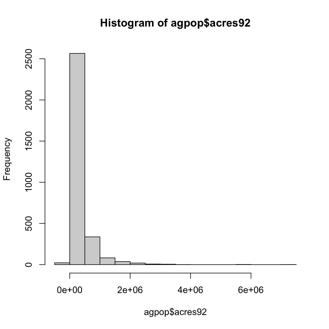
agpop_AK  <- agpop [agpop$state == "AK", ]

agpop_AK <- subset (agpop, state == "AK")

agpop_W <- subset (agpop, region == "W")

agpop_largefarm <- subset (agpop, largef92 > 10)


hist (agpop$acres92)

Produce Plots

Code

#pdf ("hist_acres92.pdf") ## use this command and dev.off to save the output to a file
hist (agpop$acres92)

Code

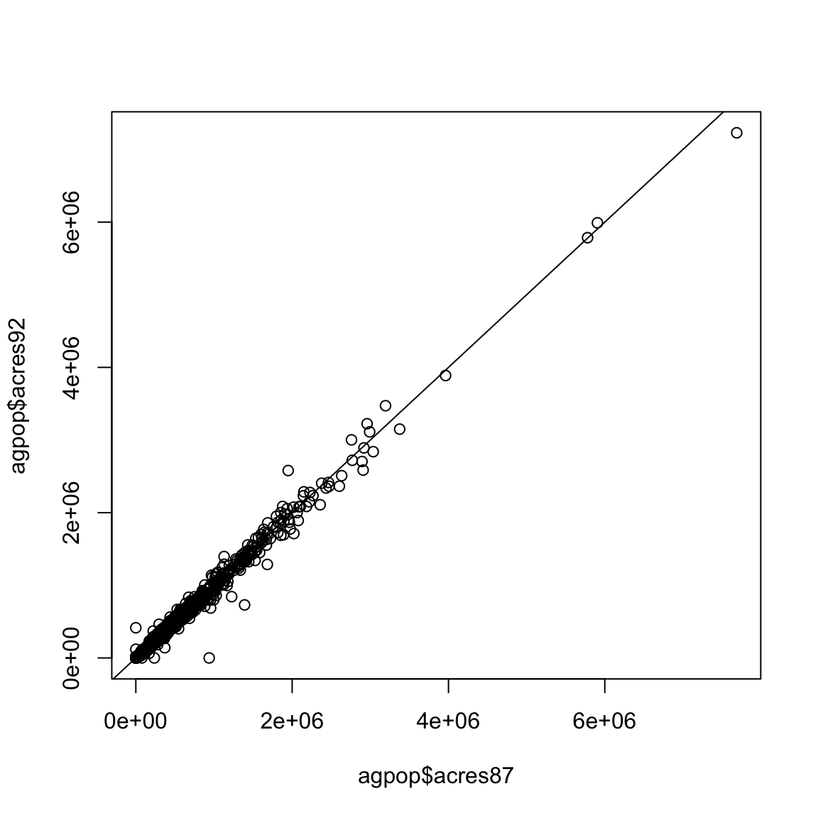
#dev.off()

#jpeg ("agpop_acres_87v92.jpg")

plot (agpop$acres87, agpop$acres92)
abline (a = 0, b = 1)

Code

#dev.off()## this is used to close the jpeg file

2.3 Create your own function

Code

### data is a matrix or data.frame
means_col <- function (data)
{
    n <- ncol (data)
    cmeans <- rep (NA, n)
    for (j in 1:n)
    {
        cmeans[j] <- mean (data[,j])
        
    }
    cmeans
}

### apply function
means_col (agpop[, 3:13])

 [1] 306676.97141 313016.37817 320193.69298    625.50357    678.28428
 [6]    728.06238     56.17674     54.86160     52.62248     54.09227
[11]     59.53769

Code

### R built-in function
colMeans (agpop[, 3:13])

     acres92      acres87      acres82      farms92      farms87      farms82 
306676.97141 313016.37817 320193.69298    625.50357    678.28428    728.06238 
    largef92     largef87     largef82     smallf92     smallf87 
    56.17674     54.86160     52.62248     54.09227     59.53769

2.4 Include Images Saved in An External File

Using the following R code to include your images saved in an external file.

Code

knitr::include_graphics("handwriting.png")

You can hide the above R code by setting “echo=FALSE” for the r chunk. For example, I will include the image once again as follows:

Figure 2.1: This is a figure inserted from the file called “handwriting.png”