Code
## Read data. Change the path as necessary.
## Example: bond.data <- read.csv("wire-bond.csv")
bond.data <- read.csv("wire-bond.csv")

## This will now be automatically rendered as a paged table
bond.dataNote: You must change the file paths in the read.csv() functions below to match the location of the files on your computer (for example C:\\Users\\<YourUsername>\\Documents on Windows).
## Read data. Change the path as necessary.
## Example: bond.data <- read.csv("wire-bond.csv")
bond.data <- read.csv("wire-bond.csv")
## This will now be automatically rendered as a paged table
bond.data2D Visualization
par(mfrow = c(1, 3), mar = c(5, 4, 2, 1))

## 1) length vs strength
i1 <- which(!is.na(bond.data$length) & !is.na(bond.data$strength))
plot(bond.data$length[i1], bond.data$strength[i1],
     xlab = "Wire Length", ylab = "Pull strength", pch = 19)
text(bond.data$length[i1], bond.data$strength[i1],
     labels = i1, pos = 1, offset = 0.4, cex = 0.75)

## 2) height vs strength
i2 <- which(!is.na(bond.data$height) & !is.na(bond.data$strength))
plot(bond.data$height[i2], bond.data$strength[i2],
     xlab = "Die height", ylab = "Pull strength", pch = 19)
text(bond.data$height[i2], bond.data$strength[i2],
     labels = i2, pos = 1, offset = 0.4, cex = 0.75)

## 3) height vs length
i3 <- which(!is.na(bond.data$height) & !is.na(bond.data$length))
plot(bond.data$height[i3], bond.data$length[i3],
     xlab = "Die height", ylab = "Length", pch = 19)
text(bond.data$height[i3], bond.data$length[i3],
     labels = i3, pos = 1, offset = 0.4, cex = 0.75)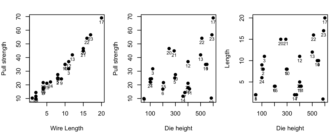
3D Visualize
library(scatterplot3d)

par(mfrow = c(1,1))
s3d <- with(bond.data, scatterplot3d(
  x = length,
  y = height,
  z = strength,
  pch = 19,
  color = "steelblue",
  main = "3D Scatterplot: Strength vs. Length and Height",
  xlab = "Length",
  ylab = "Height",
  zlab = "Strength",
  angle = 60
))

fit <- lm(strength ~ length + height, data = bond.data)
s3d$plane3d(fit, lty.box = "solid")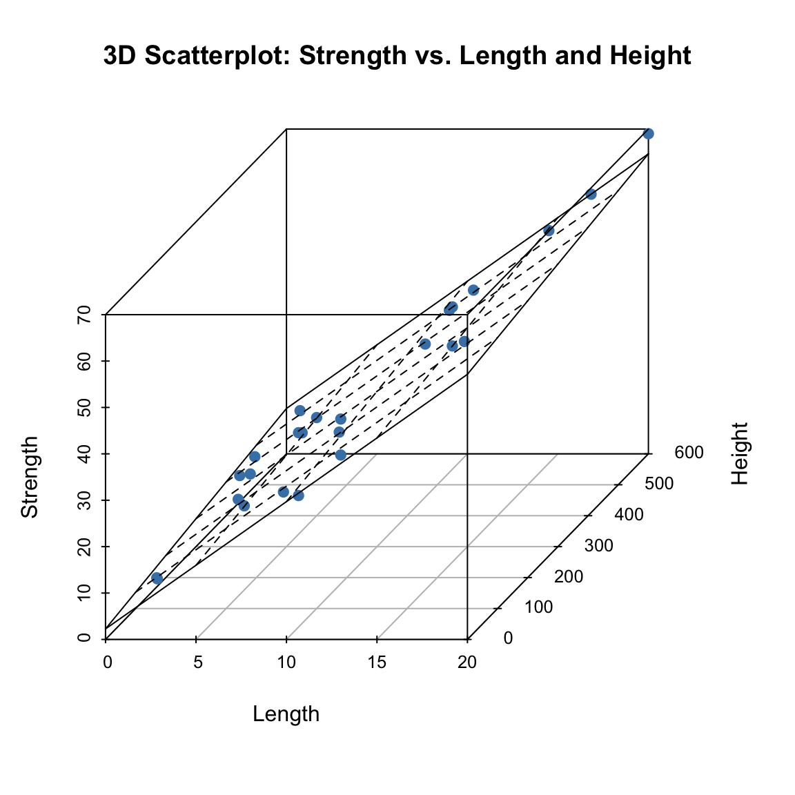
We fit a multiple linear regression model with strength as the response variable and length and height as predictors.
fit <- lm(strength ~ length + height, data = bond.data)
summary(fit)
Call:
lm(formula = strength ~ length + height, data = bond.data)

Residuals:
   Min     1Q Median     3Q    Max
-3.865 -1.542 -0.362  1.196  5.841

Coefficients:
            Estimate Std. Error t value Pr(>|t|)
(Intercept) 2.263791   1.060066   2.136 0.044099 *
length      2.744270   0.093524  29.343  < 2e-16 ***
height      0.012528   0.002798   4.477 0.000188 ***
---
Signif. codes:  0 '***' 0.001 '**' 0.01 '*' 0.05 '.' 0.1 ' ' 1

Residual standard error: 2.288 on 22 degrees of freedom
Multiple R-squared:  0.9811,    Adjusted R-squared:  0.9794
F-statistic: 572.2 on 2 and 22 DF,  p-value: < 2.2e-16
The summary provides the ANOVA F-test for overall significance, \(R^2\), adjusted \(R^2\), and t-tests for individual coefficients.
## Confidence intervals
confint(fit)
2.5 % 97.5 %
(Intercept) 0.065348613 4.46223426
length 2.550313061 2.93822623
height 0.006724246 0.01833138## Fitted values and residuals
pred <- fitted.values(fit)
e <- resid(fit)
data.frame(y = bond.data$strength, y.hat = pred, e = e)## Covariance matrix and standard errors
cov.mat <- vcov(fit)
cov.mat (Intercept) length height
(Intercept) 1.123740429 -3.921612e-02 -1.781991e-03
length -0.039216122 8.746709e-03 -9.903775e-05
height -0.001781991 -9.903775e-05 7.831149e-06data.frame(std.error = sqrt(diag(cov.mat)))The General Linear Model
The general linear model is:
\[y = X\beta + \epsilon\]
| Source | Sum of Squares | \(R^2\) | df | Mean Squares | \(F\) | SS\(_\mathrm{adj}\) | \(\hat{\sigma}^2\) | \(R^2_{\mathrm{adj}}\) |
|---|---|---|---|---|---|---|---|---|
| \(x^\top\beta\) | \(\mathrm{SSR} = \displaystyle \sum_{i=1}^n (\hat y_i - \bar y)^2\) | \(\displaystyle \frac{\mathrm{SSR}}{\mathrm{SST}}\) | \(k\) | \(\displaystyle \mathrm{MSR} = \frac{\mathrm{SSR}}{k}\) | \(\displaystyle \frac{\mathrm{MSR}}{\mathrm{MSE}}\) | \(\mathrm{SSR}_{\mathrm{adj}}\) | \(\displaystyle \hat{\sigma}^2_{x^\top\beta} = \frac{\mathrm{SSR}_{\mathrm{adj}}}{n-1}\) | \(\displaystyle \frac{\mathrm{SSR}_{\mathrm{adj}}}{\mathrm{SST}} = 1 - \frac{\mathrm{MSE}}{\mathrm{MST}}\) |
| \(\epsilon\) | \(\mathrm{SSE} = \displaystyle \sum_{i=1}^n (y_i - \hat y_i)^2\) | — | \(n-p\) | \(\displaystyle \mathrm{MSE} = \frac{\mathrm{SSE}}{n-p}\) | — | \(\mathrm{SSE}\) | \(\displaystyle \hat{\sigma}^2_{\epsilon} = \mathrm{MSE}\) | — |
| \(y\) | \(\mathrm{SST} = \displaystyle \sum_{i=1}^n (y_i - \bar y)^2\) | — | \(n-1\) | \(\displaystyle \mathrm{MST} = \frac{\mathrm{SST}}{n-1}\) | — | \(\mathrm{SST}\) | \(\displaystyle \hat{\sigma}^2_{y} = \mathrm{MST}\) | — |
Interpretation of the \(\hat{\sigma}^2\) Column
The \(\hat{\sigma}^2\) column highlights how each sum of squares corresponds to an estimated variance.
This view makes the adjusted coefficient of determination clear:
\[ R^2_{\mathrm{adj}} = 1 - \frac{\hat{\sigma}^2_\epsilon}{\hat{\sigma}^2_y} = \frac{\hat{\sigma}^2_{x^\top\beta}}{\hat{\sigma}^2_y}. \]
Hence, the adjusted \(R^2\) simply expresses the proportion of total estimated variance attributable to the fitted model \(X\beta\) rather than the residual noise \(\epsilon\).
\[ \begin{aligned} \mathrm{SST} &= \mathrm{SSR} + \mathrm{SSE}, \\ \mathrm{MST} &= \mathrm{MSE} + \frac{\mathrm{SSR}_{\mathrm{adj}}}{n-1}. \end{aligned} \]
where
\[ \mathrm{SSR}_{\mathrm{adj}} = (n-1)MST-(n-p+k)\mathrm{MSE} = \mathrm{SST}-\mathrm{SSE} - k\,\mathrm{MSE} = \mathrm{SSR} - k\,\mathrm{MSE}. \]
The quantity \(\hat{\sigma}^2\) represents the estimated variance associated with each component of the model. MSE and MST are the estimated variances of the \(\epsilon\) and \(y\) itself. However, the MSR, although called Mean Square for Regression (MSR) is NOT an estimate of the variance or sample variance of \(x^\top \beta\). The name of “mean” here is used to indicate a different thing. Its name “Mean Square” reflects that it is also an estimate estimate of noise variance \(\sigma^2\) under \(H_0\!:\,\beta = 0\):
\[ E[\mathrm{MSR} \mid H_0] = \sigma^2, \qquad E[\mathrm{MSR} \mid H_1] > \sigma^2. \]
Hence the F-statistic
\[ F = \frac{\mathrm{MSR}}{\mathrm{MSE}} \] is approximately equal to 1 subject to the variability as characterized with F-distribution with degree freedoms of \(k\) and \(n-p\). This test is to test whether any regression coefficients are not equal to 0.
\(\hat \sigma^2_{x^\top\beta}\) is an unbiased estimator of the variance of linear signal when \(x\) is a regarded as a random variable. This can be seen from the following equations: \[ E[\mathrm{SSR}] = k\,\sigma^2 + \beta^\top X^\top (I - J/n)\,X\,\beta, \qquad E[\mathrm{MSE}] = \sigma^2. \] Hence, \[ \begin{aligned} E[\mathrm{SSR}_{\mathrm{adj}}] &= E[\mathrm{SSR}] - k\,E[\mathrm{MSE}] \\ &= \beta^\top X^\top (I - J/n)\,X\,\beta \\ &= \sum_{i=1}^n (\mu_i - \bar\mu)^2, \end{aligned} \]
where \[ \begin{aligned} \mu_i &= x_i^\top \beta \\ \bar\mu &= \tfrac{1}{n}\sum_{i=1}^n \mu_i \end{aligned} \] For fixed \(X\), \(\mathrm{SSR}_{\text{adj}}/(n-1)\) equals the sample variance of the true means \(\{\mu_i\}\) over the observed design points. If the rows of \(X\) are independently sampled with covariance matrix \(\Sigma_X\) (the random-\(X\) model), then
\[ \mathbb{E}_X\!\left[\frac{\mathrm{SSR}_{\text{adj}}}{n-1}\right] = \beta^\top \Sigma_X \beta = \mathrm{Var}(x^\top \beta), \]
The decomposition of \(\hat{\sigma}^2\) is consistent with the Rao–Blackwell formula for total variance:
\[ \mathrm{Var}(y) = \mathrm{Var}\!\big(E[y \mid x]\big) + E\!\big(\mathrm{Var}[y \mid x]\big). \]
Here,
We simulate a dataset with \(n=30\) observations and consider a sequence of nested models adding groups of predictors.
Predictor Groups:
Under \(H_0\), the true coefficient for \(x_1\) is \(\beta_1 = 0\). All predictors are noise.
Under \(H_1\), \(x_1\) is a true predictor (\(\beta_1 = 2\)). The subsequent groups (\(x_2 \dots x_{20}\)) remain noise.
## Data: Weight, height and age of children
wgt <- c(64, 71, 53, 67, 55, 58, 77, 57, 56, 51, 76, 68)
hgt <- c(57, 59, 49, 62, 51, 50, 55, 48, 42, 42, 61, 57)
age <- c(8, 10, 6, 11, 8, 7, 10, 9, 10, 6, 12, 9)
child.data <- data.frame(wgt, hgt, age)fit_hgt_age <- lm(wgt ~ hgt + age, data = child.data)
summary(fit_hgt_age)
Call:
lm(formula = wgt ~ hgt + age, data = child.data)

Residuals:
    Min      1Q  Median      3Q     Max
-6.8708 -1.7004  0.3454  1.4642 10.2336

Coefficients:
            Estimate Std. Error t value Pr(>|t|)
(Intercept)   6.5530    10.9448   0.599   0.5641
hgt           0.7220     0.2608   2.768   0.0218 *
age           2.0501     0.9372   2.187   0.0565 .
---
Signif. codes:  0 '***' 0.001 '**' 0.01 '*' 0.05 '.' 0.1 ' ' 1

Residual standard error: 4.66 on 9 degrees of freedom
Multiple R-squared:   0.78, Adjusted R-squared:  0.7311
F-statistic: 15.95 on 2 and 9 DF, p-value: 0.001099fit_hgt <- lm(wgt ~ hgt, data = child.data)
summary(fit_hgt)
Call:
lm(formula = wgt ~ hgt, data = child.data)

Residuals:
    Min      1Q  Median      3Q     Max
-5.8736 -3.8973 -0.4402  2.2624 11.8375

Coefficients:
            Estimate Std. Error t value Pr(>|t|)
(Intercept)   6.1898    12.8487   0.482  0.64035
hgt           1.0722     0.2417   4.436  0.00126 **
---
Signif. codes:  0 '***' 0.001 '**' 0.01 '*' 0.05 '.' 0.1 ' ' 1

Residual standard error: 5.471 on 10 degrees of freedom
Multiple R-squared:  0.663, Adjusted R-squared:  0.6293
F-statistic: 19.67 on 1 and 10 DF, p-value: 0.001263anova(fit_hgt, fit_hgt_age)anova(fit_hgt_age)fit_age <- lm(wgt ~ age, data = child.data)
summary(fit_age)
Call:
lm(formula = wgt ~ age, data = child.data)

Residuals:
    Min      1Q  Median      3Q     Max
-11.000  -3.911   1.143   4.071  10.000

Coefficients:
            Estimate Std. Error t value Pr(>|t|)
(Intercept)  30.5714     8.6137   3.549  0.00528 **
age           3.6429     0.9551   3.814  0.00341 **
---
Signif. codes:  0 '***' 0.001 '**' 0.01 '*' 0.05 '.' 0.1 ' ' 1

Residual standard error: 6.015 on 10 degrees of freedom
Multiple R-squared:  0.5926,    Adjusted R-squared:  0.5519
F-statistic: 14.55 on 1 and 10 DF, p-value: 0.003407fit_age_hgt <- lm(wgt ~ age + hgt, data = child.data)
summary(fit_age_hgt)
Call:
lm(formula = wgt ~ age + hgt, data = child.data)

Residuals:
    Min      1Q  Median      3Q     Max
-6.8708 -1.7004  0.3454  1.4642 10.2336

Coefficients:
            Estimate Std. Error t value Pr(>|t|)
(Intercept)   6.5530    10.9448   0.599   0.5641
age           2.0501     0.9372   2.187   0.0565 .
hgt           0.7220     0.2608   2.768   0.0218 *
---
Signif. codes:  0 '***' 0.001 '**' 0.01 '*' 0.05 '.' 0.1 ' ' 1

Residual standard error: 4.66 on 9 degrees of freedom
Multiple R-squared:   0.78, Adjusted R-squared:  0.7311
F-statistic: 15.95 on 2 and 9 DF, p-value: 0.001099anova(fit_age, fit_age_hgt)anova(fit_age_hgt)fit_len_hgt <- lm(strength ~ length + height, data = bond.data)
fit_hgt_len <- lm(strength ~ height+length, data = bond.data)
anova(fit_len_hgt)anova(fit_hgt_len)summary(fit_hgt_len)
Call:
lm(formula = strength ~ height + length, data = bond.data)

Residuals:
   Min     1Q Median     3Q    Max
-3.865 -1.542 -0.362  1.196  5.841

Coefficients:
            Estimate Std. Error t value Pr(>|t|)
(Intercept) 2.263791   1.060066   2.136 0.044099 *
height      0.012528   0.002798   4.477 0.000188 ***
length      2.744270   0.093524  29.343  < 2e-16 ***
---
Signif. codes:  0 '***' 0.001 '**' 0.01 '*' 0.05 '.' 0.1 ' ' 1

Residual standard error: 2.288 on 22 degrees of freedom
Multiple R-squared:  0.9811,    Adjusted R-squared:  0.9794
F-statistic: 572.2 on 2 and 22 DF, p-value: < 2.2e-16summary(fit_len_hgt)
Call:
lm(formula = strength ~ length + height, data = bond.data)

Residuals:
   Min     1Q Median     3Q    Max
-3.865 -1.542 -0.362  1.196  5.841

Coefficients:
            Estimate Std. Error t value Pr(>|t|)
(Intercept) 2.263791   1.060066   2.136 0.044099 *
length      2.744270   0.093524  29.343  < 2e-16 ***
height      0.012528   0.002798   4.477 0.000188 ***
---
Signif. codes:  0 '***' 0.001 '**' 0.01 '*' 0.05 '.' 0.1 ' ' 1

Residual standard error: 2.288 on 22 degrees of freedom
Multiple R-squared:  0.9811,    Adjusted R-squared:  0.9794
F-statistic: 572.2 on 2 and 22 DF, p-value: < 2.2e-16predict(fit, newdata = data.frame(length = 8, height = 275),
interval = "confidence", level = 0.95) fit lwr upr
1 27.6631 26.66324 28.66296predict(fit, newdata = data.frame(length = 8, height = 275),
interval = "prediction", level = 0.95) fit lwr upr
1 27.6631 22.81378 32.51241residuals_df <- data.frame(
hat_values = hatvalues(fit),
ordinary_resid = resid(fit),
standardized_resid = resid(fit) / sigma(fit),
studentized_internal = rstandard(fit),
studentized_external = rstudent(fit)
)
residuals_dfn <- nrow(bond.data)
r <- rstudent(fit)
y.hat <- fitted.values(fit)
par(mfrow = c(2, 3), mar = c(4, 4, 2, 1))
qqnorm(r, main = "Normal Q-Q Plot"); qqline(r)
plot(y.hat, r, xlab = "Fitted values", ylab = "Studentized Residuals"); abline(h = 0)
plot(1:n, r, xlab = "Observation Number", ylab = "Studentized Residuals"); abline(h = 0)
plot(bond.data$length, r, xlab = "Wire Length", ylab = "Studentized Residuals"); abline(h = 0)
plot(bond.data$height, r, xlab = "Die Height", ylab = "Studentized Residuals"); abline(h = 0)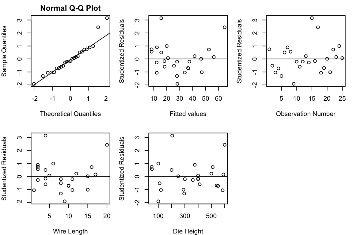
influence_df <- data.frame(dffits = dffits(fit),
                           cook.D = cooks.distance(fit),
                           dfbetas(fit))
influence_dfolsrr Package## install.packages("olsrr") # Run once if needed
library(olsrr)
ols_plot_cooksd_chart(fit)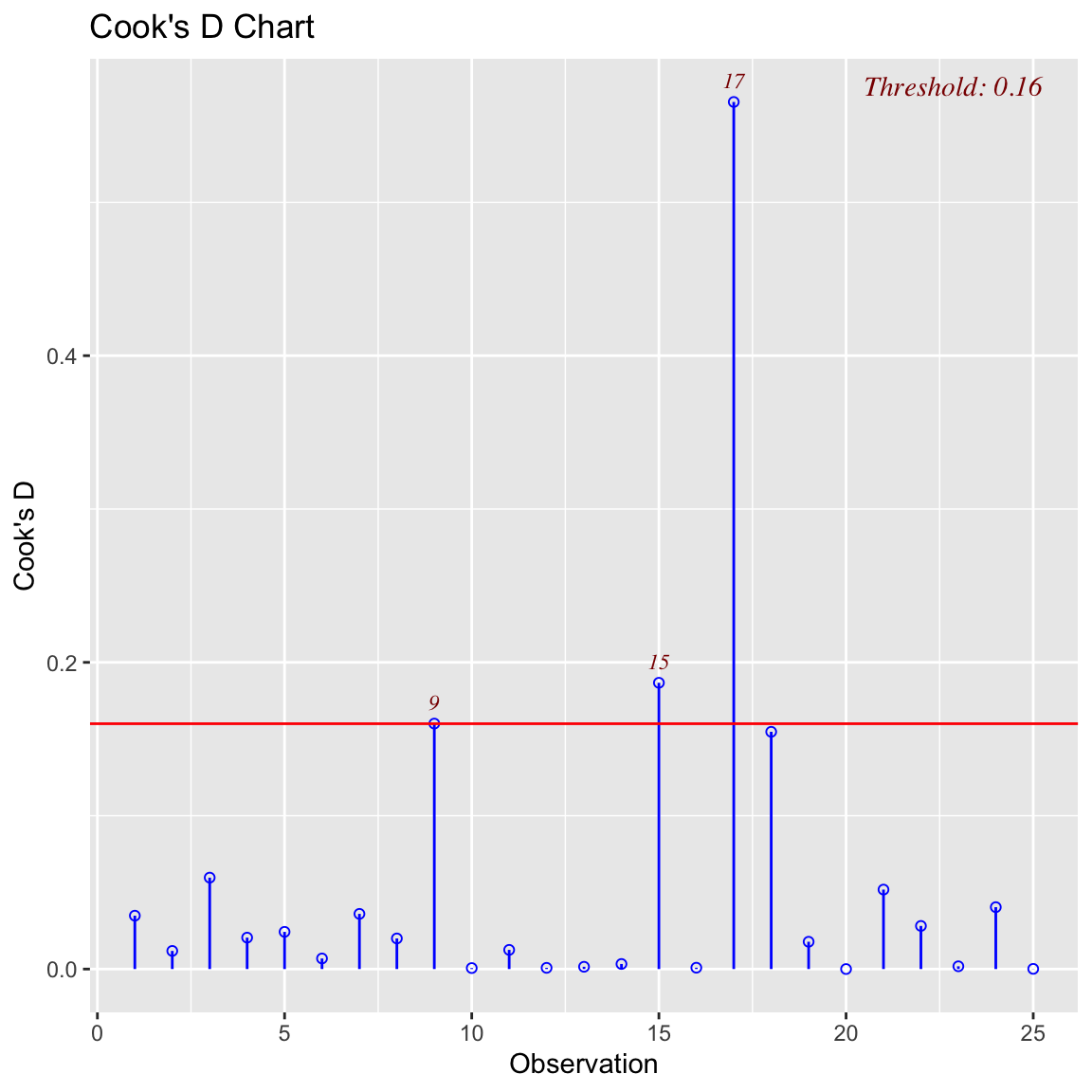
ols_plot_dffits(fit)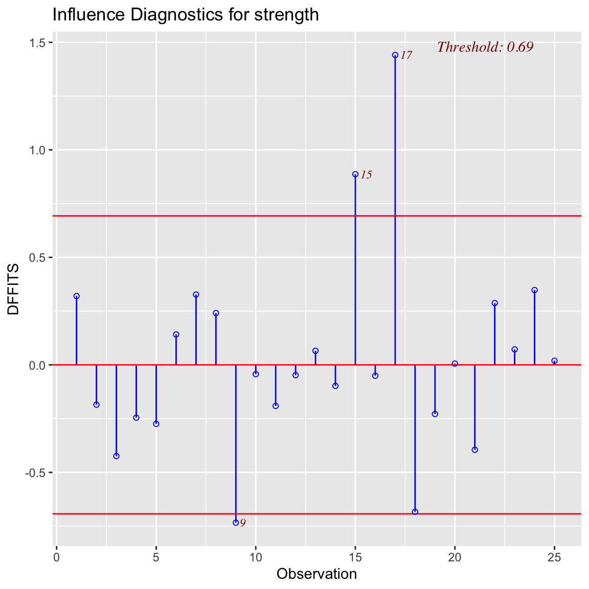
ols_plot_dfbetas(fit)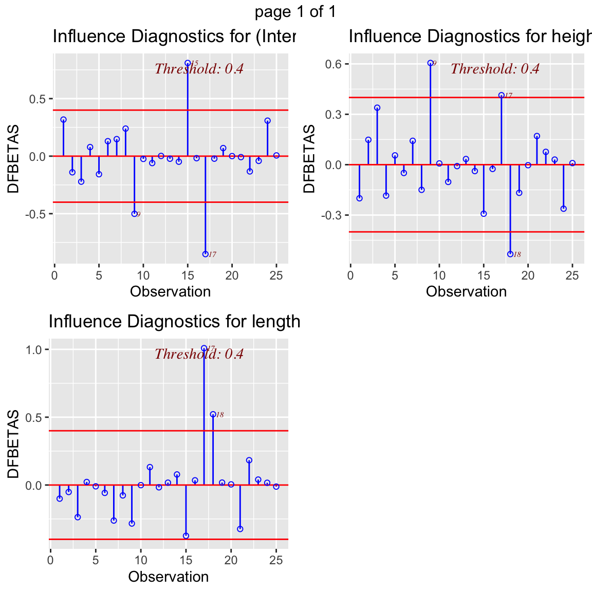
y <- c(1.81, 1.70, 1.65, 1.55, 1.48, 1.40, 1.30, 1.26, 1.24, 1.21, 1.20, 1.18)
x <- c(20, 25, 30, 35, 40, 50, 60, 65, 70, 75, 80, 90)
fit_poly <- lm(y ~ x + I(x^2))
summary(fit_poly)
Call:
lm(formula = y ~ x + I(x^2))

Residuals:
       Min         1Q     Median         3Q        Max
-0.0174763 -0.0065087  0.0001297  0.0071482  0.0151887

Coefficients:
              Estimate Std. Error t value Pr(>|t|)
(Intercept)  2.198e+00  2.255e-02   97.48 6.38e-15 ***
x           -2.252e-02  9.424e-04  -23.90 1.88e-09 ***
I(x^2)       1.251e-04  8.658e-06   14.45 1.56e-07 ***
---
Signif. codes:  0 '***' 0.001 '**' 0.01 '*' 0.05 '.' 0.1 ' ' 1

Residual standard error: 0.01219 on 9 degrees of freedom
Multiple R-squared:  0.9975,    Adjusted R-squared:  0.9969
F-statistic: 1767 on 2 and 9 DF, p-value: 2.096e-12plot(x, y, xlab = "Lot size, x", ylab = "Average cost per unit, y")
lines(x, predict(fit_poly, newdata = data.frame(x = x)), type = "l")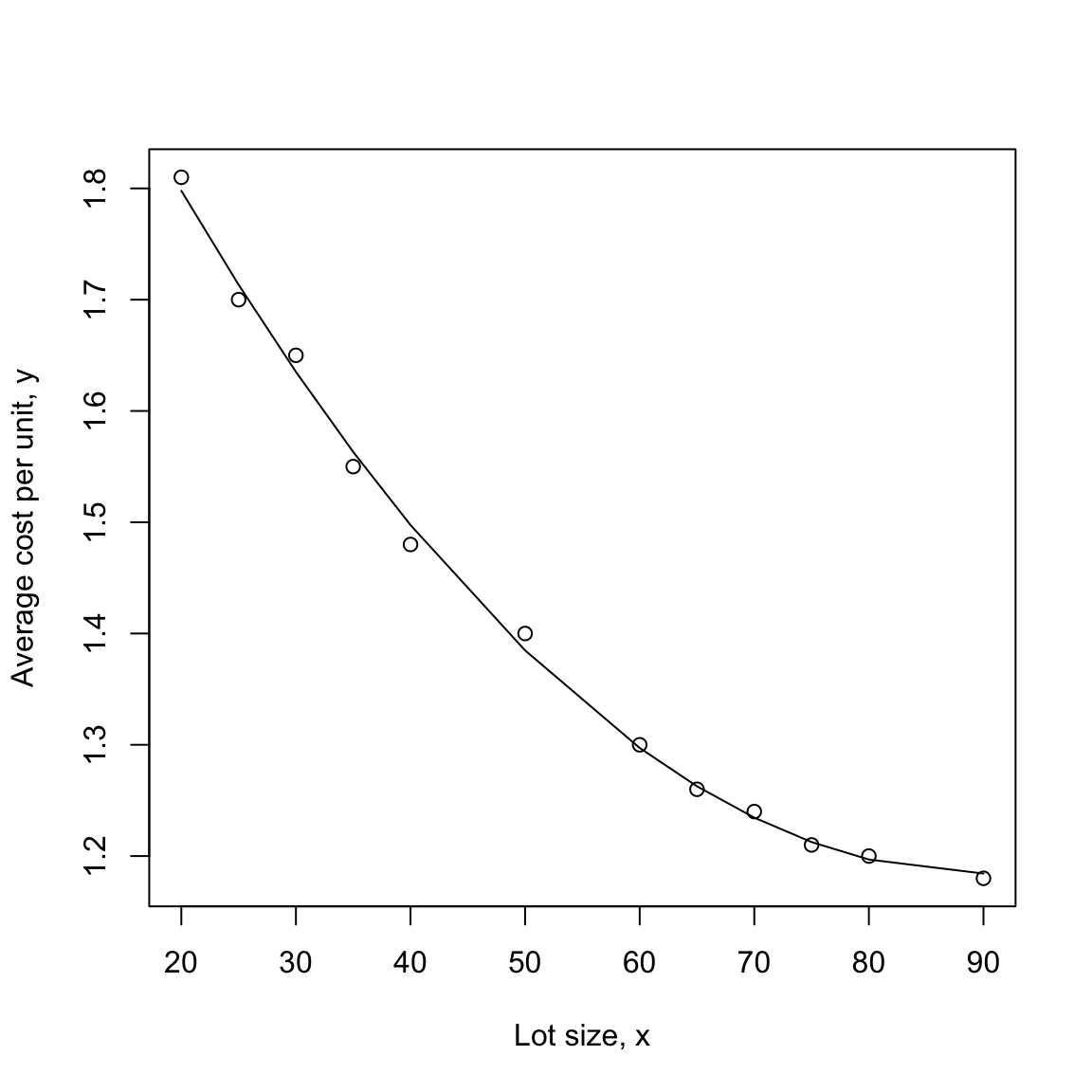
fit1 <- lm(y ~ x)
anova(fit1, fit_poly)Investigate the common observation that males tend to have higher blood pressure than females of similar age.
## Note: Update this path to your local file location
sbpdata <- read.csv("sbpdata.csv")
sbpdata## Ensure sex is a factor (labels will appear in the legend)
sbpdata$sex <- as.factor(sbpdata$sex)
## Fit (you already have this)
fit.age <- lm(sbp ~ age, data = sbpdata)
## Generate predictions over the observed age range
new_age <- seq(min(sbpdata$age, na.rm = TRUE),
max(sbpdata$age, na.rm = TRUE),
length.out = 200)
pred <- predict(fit.age, newdata = data.frame(age = new_age))
## Simple palette for the sex levels (works for 1–3 levels; expand if needed)
lev <- levels(sbpdata$sex)
cols <- setNames(c("steelblue3", "tomato3", "darkorchid3")[seq_along(lev)], lev)
## Scatter plot with colored points by sex
plot(sbp ~ age, data = sbpdata,
col = cols[sbpdata$sex], pch = 16,
xlab = "Age", ylab = "Systolic BP")
## Add predicted line
lines(new_age, pred, lwd = 2)
## Legend
legend("topleft", legend = lev, col = cols[lev], pch = 16, bty = "n", title = "Sex")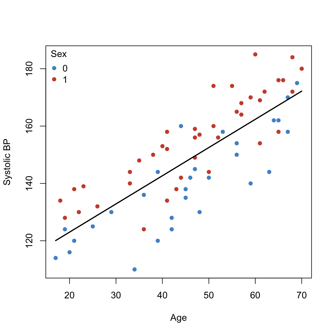
data.frame(model.matrix(fit.age)) print(anova(fit.age))Analysis of Variance Table
Response: sbp
Df Sum Sq Mean Sq F value Pr(>F)
age 1 14951.3 14951.3 121.27 < 2.2e-16 ***
Residuals 67 8260.5 123.3
---
Signif. codes: 0 '***' 0.001 '**' 0.01 '*' 0.05 '.' 0.1 ' ' 1## Parallelism: H0: beta3=0 (Sex has additive effect)
fit.agePLUSsex <- lm(sbp ~ age + sex, data = sbpdata)
## Ensure sex is a factor for labeling/colors
sbpdata$sex <- factor(sbpdata$sex)
## Fit (additive: parallelism)
fit.agePLUSsex <- lm(sbp ~ age + sex, data = sbpdata)
## X-range and palette
ages <- seq(min(sbpdata$age, na.rm = TRUE),
max(sbpdata$age, na.rm = TRUE),
length.out = 200)
lev <- levels(sbpdata$sex)
cols <- setNames(c("steelblue3", "tomato3", "darkorchid3")[seq_along(lev)], lev)
## Scatter with colored points by sex
plot(sbp ~ age, data = sbpdata,
col = cols[sbpdata$sex], pch = 16,
xlab = "Age", ylab = "Systolic BP")
## Parallel fitted lines: one per sex (same slope, different intercepts)
for (sx in lev) {
nd <- data.frame(age = ages, sex = factor(sx, levels = lev))
yhat <- predict(fit.agePLUSsex, newdata = nd)
lines(ages, yhat, col = cols[sx], lwd = 2)
}
## Legend
legend("topleft", legend = lev, col = cols[lev], pch = 16, lwd = 2, bty = "n", title = "Sex")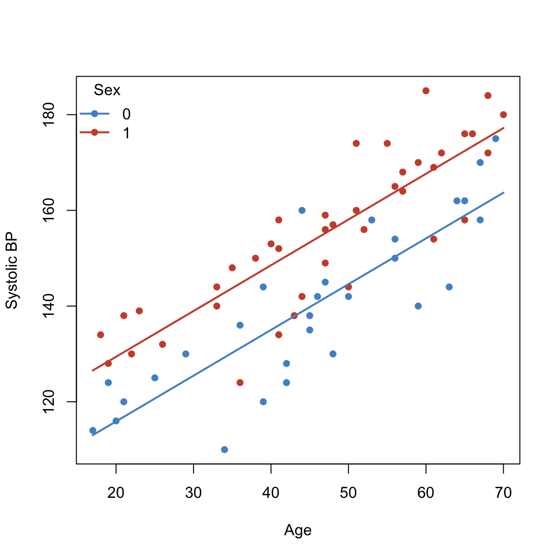
data.frame(model.matrix(fit.agePLUSsex))print(anova(fit.age, fit.agePLUSsex))Analysis of Variance Table
Model 1: sbp ~ age
Model 2: sbp ~ age + sex
Res.Df RSS Df Sum of Sq F Pr(>F)
1 67 8260.5
2 66 5202.0 1 3058.5 38.805 3.701e-08 ***
---
Signif. codes: 0 '***' 0.001 '**' 0.01 '*' 0.05 '.' 0.1 ' ' 1## Make sure sex is a factor (for colors/legend)
sbpdata$sex <- factor(sbpdata$sex)
## Fit (interaction: different slopes by sex)
fit.age.TIMES.sex <- lm(sbp ~ age + sex + age:sex, data = sbpdata)
## Age grid and palette
ages <- seq(min(sbpdata$age, na.rm = TRUE),
max(sbpdata$age, na.rm = TRUE),
length.out = 200)
lev <- levels(sbpdata$sex)
cols <- setNames(c("steelblue3", "tomato3", "darkorchid3")[seq_along(lev)], lev)
## Scatter: color points by sex
plot(sbp ~ age, data = sbpdata,
col = cols[sbpdata$sex], pch = 16,
xlab = "Age", ylab = "Systolic BP")
## Fitted lines: one per sex (different slopes allowed)
for (sx in lev) {
nd <- data.frame(age = ages, sex = factor(sx, levels = lev))
yhat <- predict(fit.age.TIMES.sex, newdata = nd)
lines(ages, yhat, col = cols[sx], lwd = 2)
}
## Legend
legend("topleft", legend = lev, col = cols[lev], pch = 16, lwd = 2, bty = "n", title = "Sex")
Model Matrix and ANOVA
data.frame(model.matrix(fit.age.TIMES.sex))summary(fit.age.TIMES.sex)
Call:
lm(formula = sbp ~ age + sex + age:sex, data = sbpdata)

Residuals:
    Min      1Q  Median      3Q     Max
-20.647  -3.410   1.254   4.314  21.153

Coefficients:
            Estimate Std. Error t value Pr(>|t|)
(Intercept) 97.07708    5.17046  18.775  < 2e-16 ***
age          0.94932    0.10864   8.738 1.43e-12 ***
sex1        12.96144    7.01172   1.849   0.0691 .
age:sex1     0.01203    0.14519   0.083   0.9342
---
Signif. codes:  0 '***' 0.001 '**' 0.01 '*' 0.05 '.' 0.1 ' ' 1

Residual standard error: 8.946 on 65 degrees of freedom
Multiple R-squared:  0.7759,    Adjusted R-squared:  0.7656
F-statistic: 75.02 on 3 and 65 DF, p-value: < 2.2e-16print(anova(fit.age,fit.agePLUSsex,fit.age.TIMES.sex))Analysis of Variance Table
Model 1: sbp ~ age
Model 2: sbp ~ age + sex
Model 3: sbp ~ age + sex + age:sex
Res.Df RSS Df Sum of Sq F Pr(>F)
1 67 8260.5
2 66 5202.0 1 3058.52 38.2210 4.692e-08 ***
3 65 5201.4 1 0.55 0.0069 0.9342
---
Signif. codes: 0 '***' 0.001 '**' 0.01 '*' 0.05 '.' 0.1 ' ' 1## Make sure sex is a factor (for colors/legend)
sbpdata$sex <- factor(sbpdata$sex)
## Fit (interaction: different slopes by sex)
fit.equal.intercept <- lm(sbp ~ age + age:sex, data = sbpdata)
## Age grid and palette
ages <- seq(min(sbpdata$age, na.rm = TRUE),
max(sbpdata$age, na.rm = TRUE),
length.out = 200)
lev <- levels(sbpdata$sex)
cols <- setNames(c("steelblue3", "tomato3", "darkorchid3")[seq_along(lev)], lev)
## Scatter: color points by sex
plot(sbp ~ age, data = sbpdata,
col = cols[sbpdata$sex], pch = 16,
xlab = "Age", ylab = "Systolic BP")
## Fitted lines: one per sex (different slopes allowed)
for (sx in lev) {
nd <- data.frame(age = ages, sex = factor(sx, levels = lev))
yhat <- predict(fit.equal.intercept, newdata = nd)
lines(ages, yhat, col = cols[sx], lwd = 2)
}
## Legend
legend("topleft", legend = lev, col = cols[lev], pch = 16, lwd = 2, bty = "n", title = "Sex")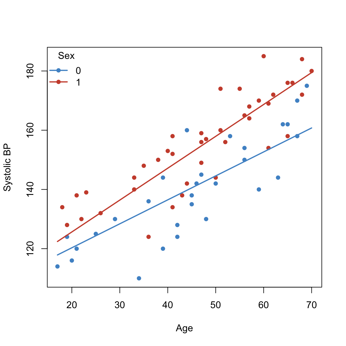
fit.int <- lm(sbp ~ 1, data = sbpdata)
fit.sex <- lm(sbp ~ sex, data = sbpdata)

print(anova(fit.int,fit.age,fit.agePLUSsex, fit.age.TIMES.sex))
Analysis of Variance Table
Model 1: sbp ~ 1
Model 2: sbp ~ age
Model 3: sbp ~ age + sex
Model 4: sbp ~ age + sex + age:sex
Res.Df RSS Df Sum of Sq F Pr(>F)
1 68 23211.8
2 67 8260.5 1 14951.3 186.8390 < 2.2e-16 ***
3 66 5202.0 1 3058.5 38.2210 4.692e-08 ***
4 65 5201.4 1 0.5 0.0069 0.9342
---
Signif. codes: 0 '***' 0.001 '**' 0.01 '*' 0.05 '.' 0.1 ' ' 1print(anova(fit.int,fit.age,fit.equal.intercept, fit.age.TIMES.sex))Analysis of Variance Table
Model 1: sbp ~ 1
Model 2: sbp ~ age
Model 3: sbp ~ age + age:sex
Model 4: sbp ~ age + sex + age:sex
Res.Df RSS Df Sum of Sq F Pr(>F)
1 68 23211.8
2 67 8260.5 1 14951.3 186.8390 < 2.2e-16 ***
3 66 5474.9 1 2785.6 34.8107 1.437e-07 ***
4 65 5201.4 1 273.4 3.4171 0.06907 .
---
Signif. codes: 0 '***' 0.001 '**' 0.01 '*' 0.05 '.' 0.1 ' ' 1print(anova(fit.int,fit.sex,fit.agePLUSsex, fit.age.TIMES.sex))Analysis of Variance Table
Model 1: sbp ~ 1
Model 2: sbp ~ sex
Model 3: sbp ~ age + sex
Model 4: sbp ~ age + sex + age:sex
Res.Df RSS Df Sum of Sq F Pr(>F)
1 68 23211.8
2 67 19282.5 1 3929.2 49.1017 1.684e-09 ***
3 66 5202.0 1 14080.6 175.9583 < 2.2e-16 ***
4 65 5201.4 1 0.5 0.0069 0.9342
---
Signif. codes: 0 '***' 0.001 '**' 0.01 '*' 0.05 '.' 0.1 ' ' 1summary(fit.age)
Call:
lm(formula = sbp ~ age, data = sbpdata)

Residuals:
    Min      1Q  Median      3Q     Max
-26.782  -7.632   1.968   8.201  22.651

Coefficients:
             Estimate Std. Error t value Pr(>|t|)
(Intercept) 103.34905    4.33190   23.86   <2e-16 ***
age           0.98333    0.08929   11.01   <2e-16 ***
---
Signif. codes:  0 '***' 0.001 '**' 0.01 '*' 0.05 '.' 0.1 ' ' 1

Residual standard error: 11.1 on 67 degrees of freedom
Multiple R-squared:  0.6441,    Adjusted R-squared:  0.6388
F-statistic: 121.3 on 1 and 67 DF, p-value: < 2.2e-16summary(fit.equal.intercept)
Call:
lm(formula = sbp ~ age + age:sex, data = sbpdata)

Residuals:
     Min       1Q   Median       3Q      Max
-21.6338  -4.3067   0.9922   4.9819  20.2753

Coefficients:
             Estimate Std. Error t value Pr(>|t|)
(Intercept) 104.12501    3.55578  29.283  < 2e-16 ***
age           0.80908    0.07918  10.219 3.14e-15 ***
age:sex1      0.26705    0.04608   5.795 2.09e-07 ***
---
Signif. codes:  0 '***' 0.001 '**' 0.01 '*' 0.05 '.' 0.1 ' ' 1

Residual standard error: 9.108 on 66 degrees of freedom
Multiple R-squared:  0.7641,    Adjusted R-squared:  0.757
F-statistic: 106.9 on 2 and 66 DF, p-value: < 2.2e-16summary(fit.agePLUSsex)
Call:
lm(formula = sbp ~ age + sex, data = sbpdata)

Residuals:
    Min      1Q  Median      3Q     Max
-20.705  -3.299   1.248   4.325  21.160

Coefficients:
            Estimate Std. Error t value Pr(>|t|)
(Intercept) 96.77353    3.62085  26.727  < 2e-16 ***
age          0.95606    0.07153  13.366  < 2e-16 ***
sex1        13.51345    2.16932   6.229  3.7e-08 ***
---
Signif. codes:  0 '***' 0.001 '**' 0.01 '*' 0.05 '.' 0.1 ' ' 1

Residual standard error: 8.878 on 66 degrees of freedom
Multiple R-squared:  0.7759,    Adjusted R-squared:  0.7691
F-statistic: 114.2 on 2 and 66 DF, p-value: < 2.2e-16summary(fit.age.TIMES.sex)
Call:
lm(formula = sbp ~ age + sex + age:sex, data = sbpdata)

Residuals:
    Min      1Q  Median      3Q     Max
-20.647  -3.410   1.254   4.314  21.153

Coefficients:
            Estimate Std. Error t value Pr(>|t|)
(Intercept) 97.07708    5.17046  18.775  < 2e-16 ***
age          0.94932    0.10864   8.738 1.43e-12 ***
sex1        12.96144    7.01172   1.849   0.0691 .
age:sex1     0.01203    0.14519   0.083   0.9342
---
Signif. codes:  0 '***' 0.001 '**' 0.01 '*' 0.05 '.' 0.1 ' ' 1

Residual standard error: 8.946 on 65 degrees of freedom
Multiple R-squared:  0.7759,    Adjusted R-squared:  0.7656
F-statistic: 75.02 on 3 and 65 DF, p-value: < 2.2e-16library(olsrr)
## Note: Update this path to your local file location
wine <- read.csv("wine.csv")
model.wine <- lm(quality ~ ., data = wine)ols_step_best_subset(model.wine) Best Subsets Regression
-------------------------------------------------
Model Index Predictors
-------------------------------------------------
1 flavor
2 flavor oakiness
3 aroma flavor oakiness
4 clarity aroma flavor oakiness
5 clarity aroma body flavor oakiness
-------------------------------------------------
Subsets Regression Summary
-------------------------------------------------------------------------------------------------------------------------------
Adj. Pred
Model R-Square R-Square R-Square C(p) AIC SBIC SBC MSEP FPE HSP APC
-------------------------------------------------------------------------------------------------------------------------------
1 0.6242 0.6137 0.5868 9.0436 130.0214 21.6859 134.9341 61.4102 1.7010 0.0462 0.4176
2 0.6611 0.6417 0.6058 6.8132 128.0901 20.1242 134.6404 57.0033 1.6171 0.0441 0.3970
3 0.7038 0.6776 0.6379 3.9278 124.9781 18.0702 133.1661 51.3383 1.4906 0.0409 0.3659
4 0.7147 0.6801 0.6102 4.6747 125.5480 19.2854 135.3736 50.9872 1.5143 0.0418 0.3717
5 0.7206 0.6769 0.587 6.0000 126.7552 21.0956 138.2183 51.5452 1.5649 0.0436 0.3842
-------------------------------------------------------------------------------------------------------------------------------
AIC: Akaike Information Criteria
SBIC: Sawa's Bayesian Information Criteria
SBC: Schwarz Bayesian Criteria
MSEP: Estimated error of prediction, assuming multivariate normality
FPE: Final Prediction Error
HSP: Hocking's Sp
APC: Amemiya Prediction Criteria ## Backward Elimination (alpha_out = 0.1)
ols_step_backward_p(model.wine, p_val = 0.1)
                             Stepwise Summary
------------------------------------------------------------------------
Step    Variable        AIC        SBC       SBIC       R2       Adj. R2
------------------------------------------------------------------------
 0      Full Model    126.755    138.218    21.096    0.72060    0.67694
 1      body          125.548    135.374    19.285    0.71471    0.68013
 2      clarity       124.978    133.166    18.070    0.70377    0.67763
------------------------------------------------------------------------

Final Model Output
------------------

                         Model Summary
---------------------------------------------------------------
R                       0.839       RMSE                 1.098
R-Squared               0.704       MSE                  1.207
Adj. R-Squared          0.678       Coef. Var            9.338
Pred R-Squared          0.638       AIC                124.978
MAE                     0.868       SBC                133.166
---------------------------------------------------------------
 RMSE: Root Mean Square Error
 MSE: Mean Square Error
 MAE: Mean Absolute Error
 AIC: Akaike Information Criteria
 SBC: Schwarz Bayesian Criteria

                               ANOVA
-------------------------------------------------------------------
               Sum of
              Squares        DF    Mean Square      F         Sig.
-------------------------------------------------------------------
Regression    108.935         3         36.312    26.925    0.0000
Residual       45.853        34          1.349
Total         154.788        37
-------------------------------------------------------------------

                                  Parameter Estimates
----------------------------------------------------------------------------------------
      model      Beta    Std. Error    Std. Beta      t        Sig      lower     upper
----------------------------------------------------------------------------------------
(Intercept)     6.467         1.333                  4.852    0.000     3.759     9.176
      aroma     0.580         0.262        0.307     2.213    0.034     0.047     1.113
     flavor     1.200         0.275        0.603     4.364    0.000     0.641     1.758
   oakiness    -0.602         0.264       -0.217    -2.278    0.029    -1.140    -0.065
----------------------------------------------------------------------------------------## Forward Selection (alpha_in = 0.1)
ols_step_forward_p(model.wine, p_val = 0.1)
                             Stepwise Summary
------------------------------------------------------------------------
Step    Variable        AIC        SBC       SBIC       R2       Adj. R2
------------------------------------------------------------------------
 0      Base Model    165.209    168.484    55.141    0.00000    0.00000
 1      flavor        130.021    134.934    21.686    0.62417    0.61373
 2      oakiness      128.090    134.640    20.124    0.66111    0.64175
 3      aroma         124.978    133.166    18.070    0.70377    0.67763
------------------------------------------------------------------------

Final Model Output
------------------

                         Model Summary
---------------------------------------------------------------
R                       0.839       RMSE                 1.098
R-Squared               0.704       MSE                  1.207
Adj. R-Squared          0.678       Coef. Var            9.338
Pred R-Squared          0.638       AIC                124.978
MAE                     0.868       SBC                133.166
---------------------------------------------------------------
 RMSE: Root Mean Square Error
 MSE: Mean Square Error
 MAE: Mean Absolute Error
 AIC: Akaike Information Criteria
 SBC: Schwarz Bayesian Criteria

                               ANOVA
-------------------------------------------------------------------
               Sum of
              Squares        DF    Mean Square      F         Sig.
-------------------------------------------------------------------
Regression    108.935         3         36.312    26.925    0.0000
Residual       45.853        34          1.349
Total         154.788        37
-------------------------------------------------------------------

                                  Parameter Estimates
----------------------------------------------------------------------------------------
      model      Beta    Std. Error    Std. Beta      t        Sig      lower     upper
----------------------------------------------------------------------------------------
(Intercept)     6.467         1.333                  4.852    0.000     3.759     9.176
     flavor     1.200         0.275        0.603     4.364    0.000     0.641     1.758
   oakiness    -0.602         0.264       -0.217    -2.278    0.029    -1.140    -0.065
      aroma     0.580         0.262        0.307     2.213    0.034     0.047     1.113
----------------------------------------------------------------------------------------## Stepwise Regression (alpha_in = 0.1, alpha_out = 0.1)
ols_step_both_p(model.wine, p_enter = 0.1, p_remove = 0.1)
                              Stepwise Summary
--------------------------------------------------------------------------
Step    Variable          AIC        SBC       SBIC       R2       Adj. R2
--------------------------------------------------------------------------
 0      Base Model      165.209    168.484    55.141    0.00000    0.00000
 1      flavor (+)      130.021    134.934    21.686    0.62417    0.61373
 2      oakiness (+)    128.090    134.640    20.124    0.66111    0.64175
 3      aroma (+)       124.978    133.166    18.070    0.70377    0.67763
--------------------------------------------------------------------------

Final Model Output
------------------

                         Model Summary
---------------------------------------------------------------
R                       0.839       RMSE                 1.098
R-Squared               0.704       MSE                  1.207
Adj. R-Squared          0.678       Coef. Var            9.338
Pred R-Squared          0.638       AIC                124.978
MAE                     0.868       SBC                133.166
---------------------------------------------------------------
 RMSE: Root Mean Square Error
 MSE: Mean Square Error
 MAE: Mean Absolute Error
 AIC: Akaike Information Criteria
 SBC: Schwarz Bayesian Criteria

                               ANOVA
-------------------------------------------------------------------
               Sum of
              Squares        DF    Mean Square      F         Sig.
-------------------------------------------------------------------
Regression    108.935         3         36.312    26.925    0.0000
Residual       45.853        34          1.349
Total         154.788        37
-------------------------------------------------------------------

                                  Parameter Estimates
----------------------------------------------------------------------------------------
      model      Beta    Std. Error    Std. Beta      t        Sig      lower     upper
----------------------------------------------------------------------------------------
(Intercept)     6.467         1.333                  4.852    0.000     3.759     9.176
     flavor     1.200         0.275        0.603     4.364    0.000     0.641     1.758
   oakiness    -0.602         0.264       -0.217    -2.278    0.029    -1.140    -0.065
      aroma     0.580         0.262        0.307     2.213    0.034     0.047     1.113
----------------------------------------------------------------------------------------y <- c(19, 20, 37, 39, 36, 38)
x1 <- c(4, 4, 7, 7, 7.1, 7.1)
x2 <- c(16, 16, 49, 49, 50.4, 50.4)
cor(data.frame(x1, x2)) x1 x2
x1 1.0000000 0.9999713
x2 0.9999713 1.0000000fit_multi <- lm(y ~ x1 + x2)
summary(fit_multi)
Call:
lm(formula = y ~ x1 + x2)

Residuals:
   1    2    3    4    5    6
-0.5  0.5 -1.0  1.0 -1.0  1.0

Coefficients:
            Estimate Std. Error t value Pr(>|t|)
(Intercept) -156.056    117.158  -1.332    0.275
x1            65.444     45.890   1.426    0.249
x2            -5.389      4.152  -1.298    0.285

Residual standard error: 1.225 on 3 degrees of freedom
Multiple R-squared:  0.9897,    Adjusted R-squared:  0.9829
F-statistic: 144.3 on 2 and 3 DF, p-value: 0.001043fit1_multi <- lm(y ~ x1)
summary(fit1_multi)
Call:
lm(formula = y ~ x1)

Residuals:
      1       2       3       4       5       6
-0.5260  0.4740 -0.1925  1.8075 -1.7814  0.2186

Coefficients:
            Estimate Std. Error t value Pr(>|t|)
(Intercept)  -4.0293     2.3332  -1.727    0.159
x1            5.8888     0.3762  15.654 9.73e-05 ***
---
Signif. codes:  0 '***' 0.001 '**' 0.01 '*' 0.05 '.' 0.1 ' ' 1

Residual standard error: 1.325 on 4 degrees of freedom
Multiple R-squared:  0.9839,    Adjusted R-squared:  0.9799
F-statistic: 245.1 on 1 and 4 DF, p-value: 9.725e-05ols_vif_tol(fit_multi)wine.x <- wine[, -ncol(wine)] # Assuming quality is the last column
cor(wine.x) clarity aroma body flavor oakiness
clarity 1.00000000 0.0619021 -0.3083783 -0.08515993 0.1832147
aroma 0.06190210 1.0000000 0.5489102 0.73656121 0.2016444
body -0.30837826 0.5489102 1.0000000 0.64665917 0.1521059
flavor -0.08515993 0.7365612 0.6466592 1.00000000 0.1797605
oakiness 0.18321471 0.2016444 0.1521059 0.17976051 1.0000000## VIF using olsrr (data frame output)
ols_vif_tol(model.wine)## Data: Weight, height and age of children
wgt <- c(64, 71, 53, 67, 55, 58, 77, 57, 56, 51, 76, 68)
hgt <- c(57, 59, 49, 62, 51, 50, 55, 48, 42, 42, 61, 57)
age <- c(8, 10, 6, 11, 8, 7, 10, 9, 10, 6, 12, 9)
fit_age_hgt <- lm(wgt ~ hgt + age, data = child.data)
ols_vif_tol(fit_age_hgt)