3 Simple Linear Regression

Code

require("knitr")
knitr::opts_chunk$set(
  comment = "#",
  fig.width = 6,
  fig.height = 6,
  cache = TRUE
)
set.seed(47)

options(sim_rebuild=FALSE)

3.1 Overview of Simple Linear Regression

To make the simple linear regression model concrete, let’s first visualize a simulated dataset that follows \[ Y_i = \beta_0 + \beta_1 X_i + \varepsilon_i, \qquad \varepsilon_i \sim \mathcal N(0, \sigma^2). \]

Here, \(\beta_0\) is the intercept, \(\beta_1\) is the slope, and \(\varepsilon_i\) represents random noise.

Code

set.seed(2025)
n <- 40
beta0 <- 2; beta1 <- 1.5; sigma <- 2
x <- runif(n, 0, 10)
y <- beta0 + beta1 * x + rnorm(n, 0, sigma)
dat <- data.frame(x, y)

fit <- lm(y ~ x, data = dat)

plot(x, y, pch = 19, col = "steelblue",
     xlab = "Predictor X", ylab = "Response Y",
     main = "Simulated Data with Fitted Linear Regression Line")
abline(fit, col = "red", lwd = 2)
legend("topleft", legend = c("Observed data", "Fitted line"),
       pch = c(19, NA), lty = c(NA, 1), col = c("steelblue", "red"), bty = "n")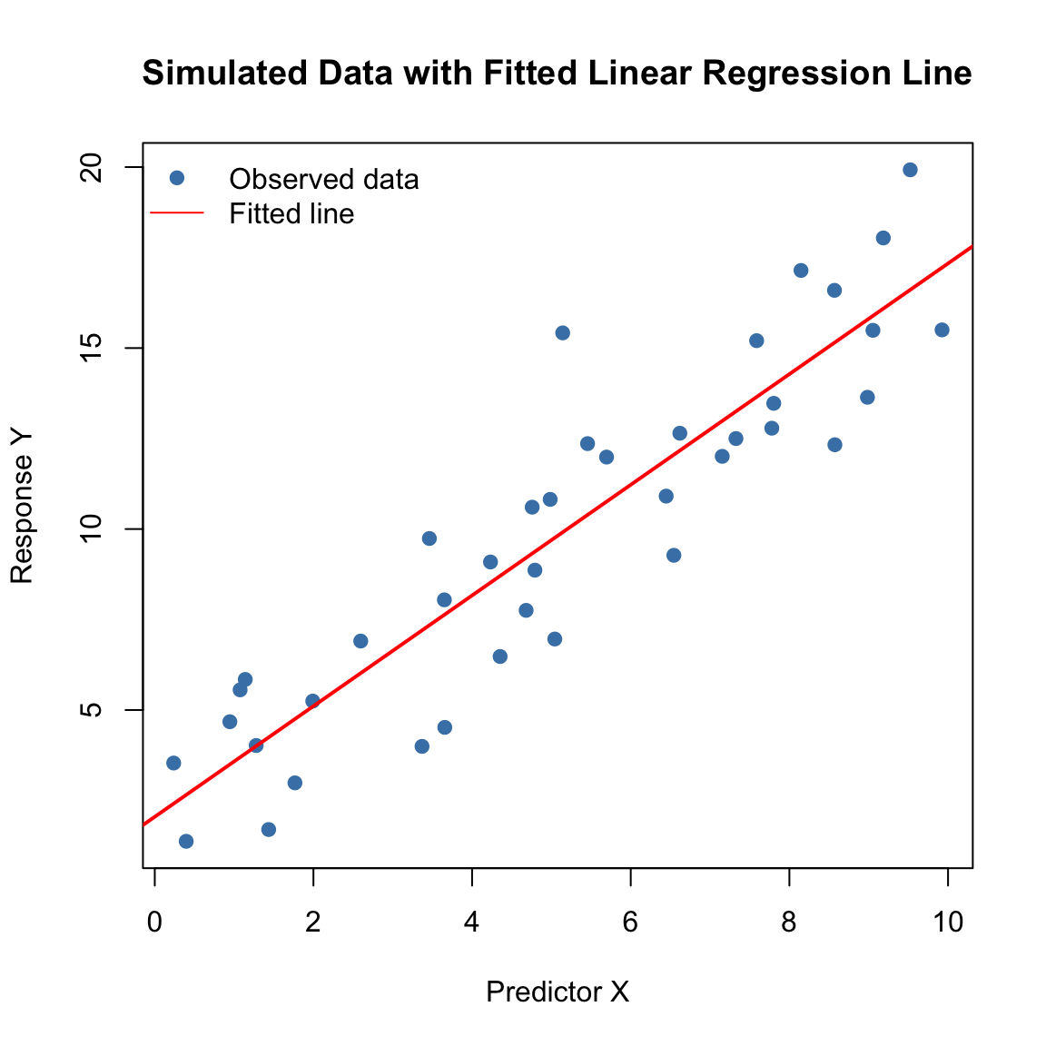

The scatterplot shows data points scattered around a line — the red line is the fitted regression model.

3.1.1 Least Squares Estimation

Goal: Find \(\hat\beta_0\) and \(\hat\beta_1\) that minimize \[ \mathrm{SSE} = \sum_{i=1}^n (y_i - \hat\beta_0 - \hat\beta_1 x_i)^2. \]

Solutions: \[ \hat\beta_1 = \frac{\sum_i (x_i - \bar x)(y_i - \bar y)}{\sum_i (x_i - \bar x)^2} = \frac{S_{xy}}{S_{xx}}, \qquad \hat\beta_0 = \bar y - \hat\beta_1\,\bar x. \]

Here \[ S_{xy} = \sum_i (x_i - \bar x)(y_i - \bar y), \qquad S_{xx} = \sum_i (x_i - \bar x)^2. \]

Shortcut (computational) formulas: \[ S_{xy} = \sum_i x_i y_i - n\,\bar x\,\bar y, \qquad S_{xx} = \sum_i x_i^2 - n\,\bar x^2. \]

Interpretation:
- \(\hat\beta_1\) measures the estimated change in \(Y\) for each unit increase in \(X\).
- \(\hat\beta_0\) represents the fitted value of \(Y\) when \(X=0\).

3.1.2 Residual and Sum of Squares Definitions

Let \(\hat y_i = \hat\beta_0 + \hat\beta_1 x_i\) and \(e_i = y_i - \hat y_i\).

Symbol	Definition	Computing Formula (in terms of \(S_{xx}, S_{xy}\), etc.)
SST	Total Sum of Squares	\(\displaystyle \sum_i (y_i - \bar y)^2 = S_{yy} = \sum_i y_i^2 - n\,\bar y^2\)
SSR	Regression Sum of Squares	\(\displaystyle \sum_i (\hat y_i - \bar y)^2 = \hat\beta_1^2 S_{xx} = \frac{S_{xy}^2}{S_{xx}}\)
SSE	Error (Residual) Sum of Squares	\(\displaystyle \sum_i (y_i - \hat y_i)^2 = S_{yy} - \frac{S_{xy}^2}{S_{xx}}\)

Identity: \[ \mathrm{SST} = \mathrm{SSR} + \mathrm{SSE}. \]

Here, \[ S_{xx} = \sum_i (x_i - \bar x)^2 = \sum_i x_i^2 - n\bar x^2, \qquad S_{yy} = \sum_i (y_i - \bar y)^2 = \sum_i y_i^2 - n\bar y^2, \qquad S_{xy} = \sum_i (x_i - \bar x)(y_i - \bar y) = \sum_i x_i y_i - n\bar x \bar y. \]

3.1.3 Coefficient of Determination (\(R^2\))

Measures the proportion of total variation in \(Y\) explained by \(X\): \[ R^2 = \frac{\mathrm{SSR}}{\mathrm{SST}} = 1 - \frac{\mathrm{SSE}}{\mathrm{SST}}. \]

Interpretation:

\(R^2 = 1\) means perfect linear fit;
\(R^2 = 0\) means the model explains none of the variation.

3.1.4 F-test for Overall Significance

Tests whether \(X\) is linearly related to \(Y\).

Hypotheses: \[ H_0: \beta_1 = 0 \quad \text{vs.} \quad H_A: \beta_1 \ne 0. \]

Test Statistic: \[ F = \frac{\text{MSR}}{\text{MSE}} = \frac{\text{SSR}/1}{\text{SSE}/(n-2)} \sim F_{1,n-2}\quad (H_0). \]

p-value approach for observe \(F^{\mathrm{obs}}\):

Given the observed statistic \(F^{\text{obs}}\) with \((1,\,n-2)\) df, \[ p-\text{value} \;=\; \Pr\!\big(F_{1,\,n-2} \ge F^{\text{obs}}\big) \;=\; \mathrm{pf}\!\big(F^{\text{obs}},\,1,\,n-2,\ \text{lower.tail}= \mathrm{FALSE}\big). \]

Code

## -- Inputs (provide these from your analysis context) -------------------------
## n   <- ...   # sample size
## SSR <- ...   # regression sum of squares
## SSE <- ...   # error sum of squares
n   <- 20
SSR <- 5
SSE <- 40




df1  <- 1
df2  <- n - 2
Fobs <- (SSR/df1) / (SSE/df2)         # observed F
pval <- pf(Fobs, df1 = df1, df2 = df2, lower.tail = FALSE)
pval

[1] 0.1509505

Code

## -- Plot F density and shade the p-value tail (with proper annotations) -------
xmax <- max(qf(0.995, df1, df2), Fobs * 1.2)  # extra space for labels
peak <- max(df(seq(0, xmax, length.out = 500), df1, df2))

## Density curve
curve(df(x, df1, df2), from = 0, to = xmax,
      xlab = "F", ylab = "Density",
      main = sprintf("F(%d, %d) density  |  observed F = %.3f", df1, df2, Fobs))

## Shade right tail (p-value region)
xs <- seq(Fobs, xmax, length.out = 300)
ys <- df(xs, df1, df2)
polygon(c(Fobs, xs, xmax), c(0, ys, 0),
        col = rgb(0, 0, 0, 0.18), border = NA)

## Vertical line at Fobs (optional visual aid)
abline(v = Fobs, lwd = 2)

## ---- Annotation for F^obs pointing to the x-axis value (Fobs, 0) -------------
x_txt_F <- Fobs + 0.06 * xmax
y_txt_F <- 0.45 * peak
arrows(x0 = x_txt_F, y0 = y_txt_F, x1 = Fobs, y1 = 0,
       length = 0.08, lwd = 1.5)
text(x_txt_F, y_txt_F,
     labels = bquote(F^{obs} == .(format(Fobs, digits = 3))),
     pos = 4)

## ---- Annotation for p-value pointing into the shaded tail --------------------
x_tip_p <- (Fobs + xmax) / 1.7
y_tip_p <- df(x_tip_p, df1, df2)
x_txt_p <- Fobs + 0.08 * xmax
y_txt_p <- 0.80 * peak
arrows(x0 = x_txt_p, y0 = y_txt_p, x1 = x_tip_p, y1 = y_tip_p,
       length = 0.08, lwd = 1.5)
text(x_txt_p, y_txt_p,
     labels = bquote(p == .(format(pval, digits = 4, scientific = TRUE))),
     pos = 4)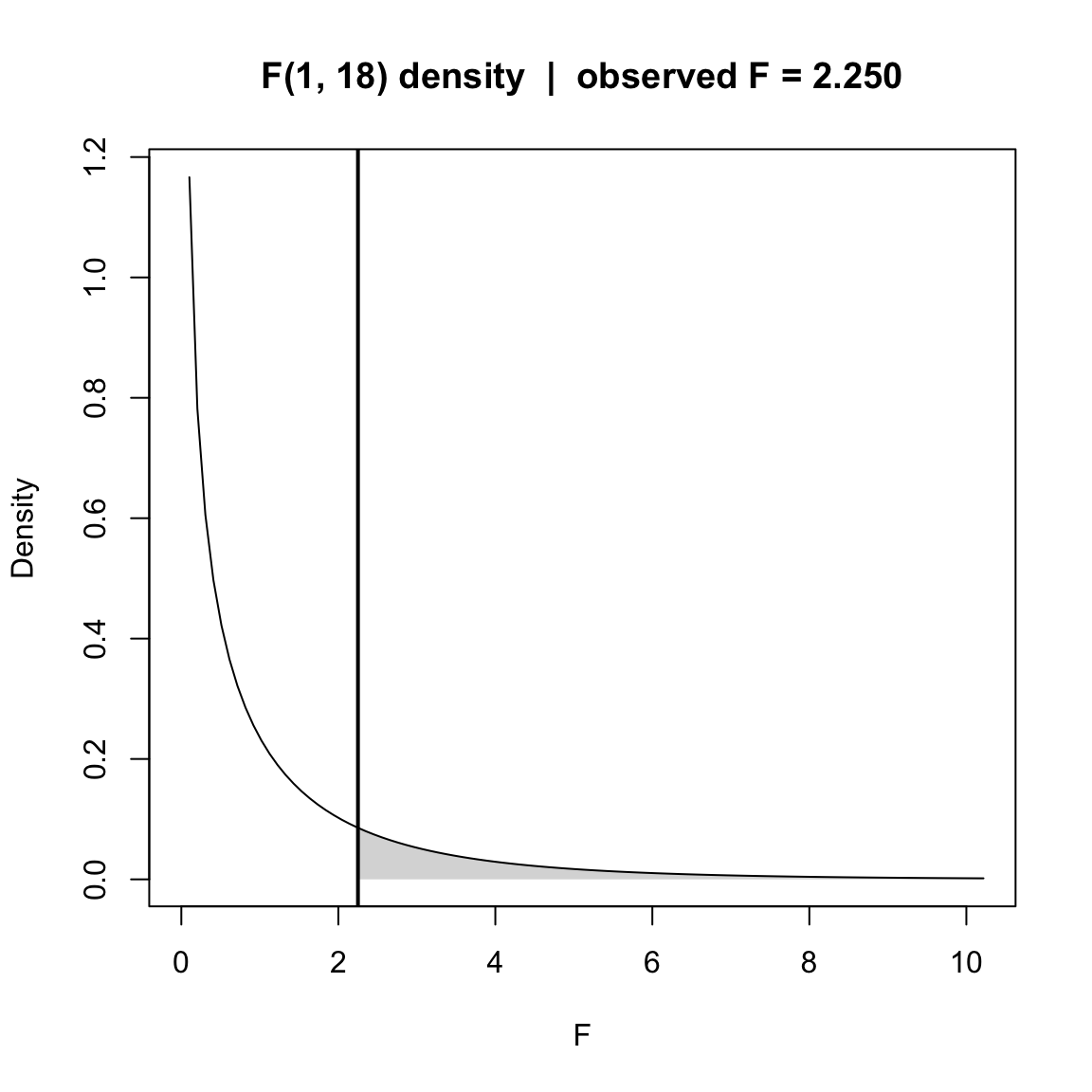

3.1.5 t-test for the Slope \(\beta_1\)

Equivalent to the \(F\)-test in simple regression since \(t^2 = F\).

Formula: \[ t = \frac{\hat\beta_1}{\operatorname{SE}(\hat\beta_1)}, \qquad \operatorname{SE}(\hat\beta_1) = \sqrt{\frac{\hat\sigma^2}{\sum_i (x_i - \bar x)^2}}, \qquad \hat\sigma^2 = \frac{\mathrm{SSE}}{n-2}. \]

Distribution: \[ t \sim t_{n-2}\quad (H_0:\beta_1=0). \]

3.1.6 Prediction for a New Case \(x_0\)

Predicted mean response: \[ \hat y(x_0) = \hat\beta_0 + \hat\beta_1 x_0. \]

95% Confidence interval for mean response: \[ \hat y(x_0) \pm t_{1-\alpha/2,,n-2}, \hat\sigma,\sqrt{\frac{1}{n} + \frac{(x_0 - \bar x)^2}{\sum_i (x_i - \bar x)^2}}. \]

95% Prediction interval for a new observation: \[ \hat y(x_0) \pm t_{1-\alpha/2,,n-2}, \hat\sigma,\sqrt{1 + \frac{1}{n} + \frac{(x_0 - \bar x)^2}{\sum_i (x_i - \bar x)^2}}. \]

Summary Cheat Sheet

Concept	Key Formula
Model	\(Y_i = \beta_0 + \beta_1 X_i + \varepsilon_i\)
LS Estimates	\(\hat\beta_1 = S_{xy}/S_{xx}\), \(\hat\beta_0 = \bar y - \hat\beta_1\bar x\)
Decomposition	\(\mathrm{SST} = \mathrm{SSR} + \mathrm{SSE}\)
\(R^2\)	\(R^2 = 1 - \mathrm{SSE}/\mathrm{SST}\)
\(F\)-test	\(F = (\mathrm{SSR}/1)/(\mathrm{SSE}/(n-2))\)
\(t\)-test	\(t = \hat\beta_1 / \operatorname{SE}(\hat\beta_1)\)
Prediction	\(\hat y(x_0) = \hat\beta_0 + \hat\beta_1 x_0\)

3.2 Example 1: Vehicle Insurance Premium (warm-up)

We examine premiums \(y\) vs. driving amount \(x\). The scatterplot hints at a downward trend.

3.2.1 Input data

Code

issu <- data.frame(
  driving = c(5, 2, 12, 9, 15, 6, 25, 16),
  premium = c(64, 87, 50, 71, 44, 56, 42, 60)
)

y <- issu$premium
x <- issu$driving
xbar <- mean(x); ybar <- mean(y); n <- length(y)

plot(x, y, xlab = "Driving", ylab = "Premium",
     main = "Vehicle Insurance: Premium vs. Driving")
abline(h = ybar, lty = 3)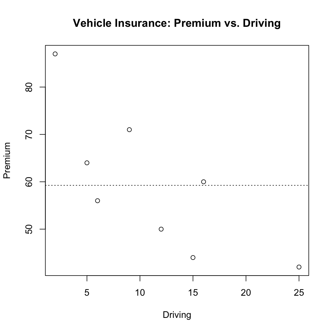

Narrative. The horizontal line at \(\bar y\) represents the intercept-only model. Any fitted line that tilts away from this must earn its keep by reducing residual variation enough to offset the loss of one degree of freedom.

3.2.2 Estimating regression coefficients

Code

fit.issu <- lm(y ~ x)
plot(x, y, xlab = "Driving", ylab = "Premium",
     main = "Fitted Simple Linear Regression")
abline(fit.issu, lwd = 2)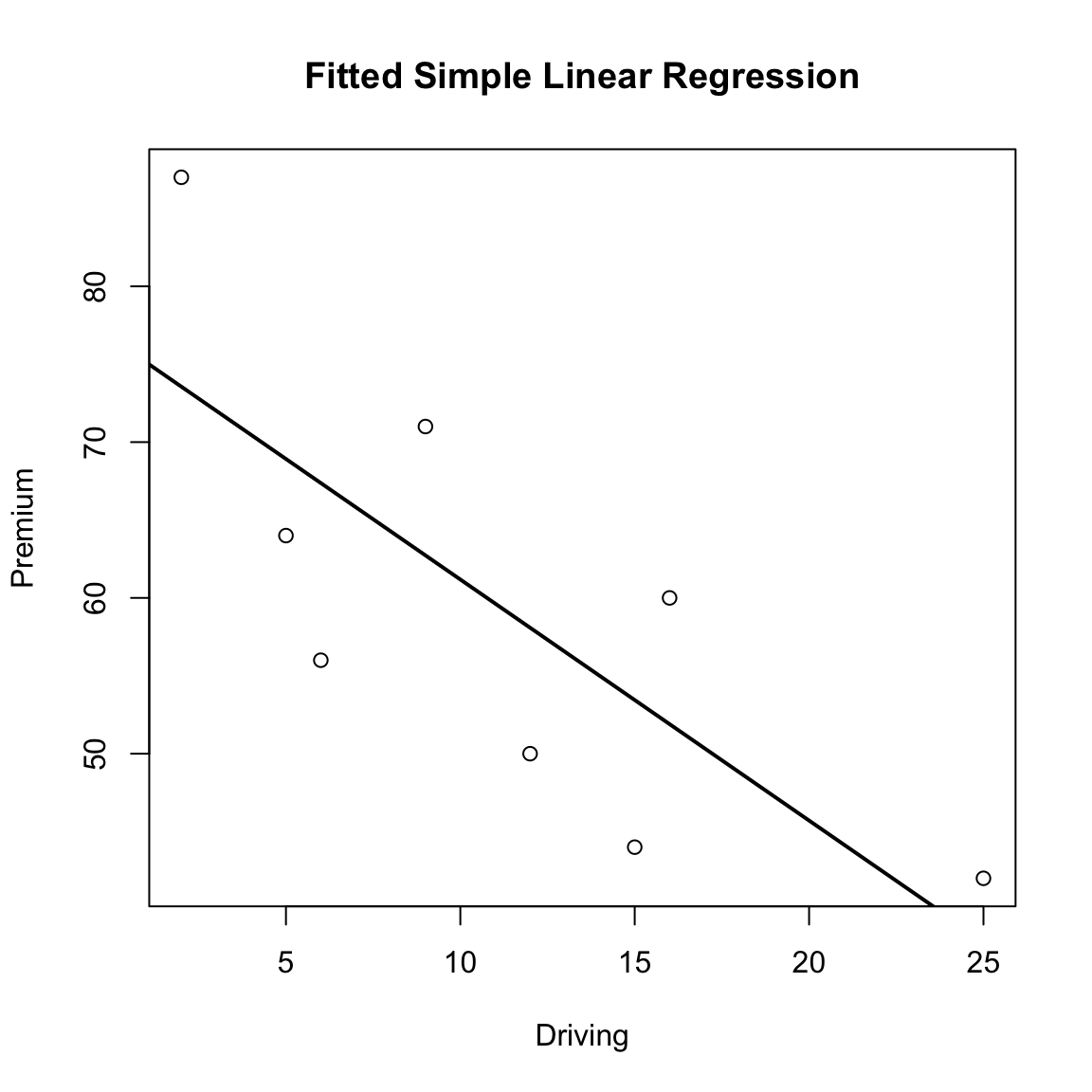

The slope estimate \(\hat\beta_1\) captures the marginal change in premium per unit of driving (units of \(y\) per unit of \(x\)). Inference on \(\beta_1\) tells us whether the pattern rises above noise.

3.2.3 Residuals and fitted values (geometry picture)

Let \(\hat y_i=\hat\beta_0+\hat\beta_1 x_i\) and \(\tilde y_i=\bar y\). Residuals are \(e_i=y_i-\hat y_i\) (model) and \(y_i-\bar y\) (null). Visualizing all three clarifies the ANOVA identity.

Code

beta0 <- coef(fit.issu)[1]
beta1 <- coef(fit.issu)[2]
fitted1 <- beta0 + beta1 * x
fitted0 <- rep(ybar, n)
residual1 <- y - fitted1
residual0 <- y - fitted0

data.frame(y, fitted0, residual0, fitted1, residual1,
           diff.fitted = fitted1 - fitted0)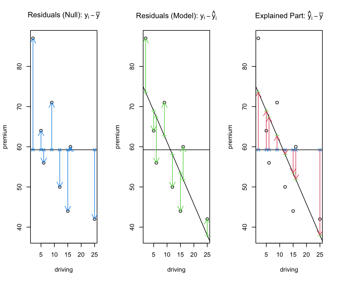

3.2.4 SST, SSR, SSE and their meanings

\(\text{SST}=\sum (y_i-\bar y)^2\) quantifies total variability around the mean.
\(\text{SSR}=\sum (\hat y_i-\bar y)^2\) is the part explained by \(x\).
\(\text{SSE}=\sum (y_i-\hat y_i)^2\) is the leftover (unexplained) variability.

Code

SST <- sum((y - fitted0)^2); SST

[1] 1557.5

Code

SSE <- sum((y - fitted1)^2); SSE

[1] 639.0065

Code

SSR <- SST - SSE; SSR

[1] 918.4935

Direct check: \(\text{SSR}=\sum(\hat y_i-\bar y)^2\).

Code

sum((fitted1 - fitted0)^2)

[1] 918.4935

3.2.5 Visual ANOVA on an RSS plot

We place the residual sum of squares against model dimension to show the trade-off between fit and df.

Code

## Recompute cleanly
SST <- sum((y - mean(y))^2)
SSE <- sum(resid(fit.issu)^2)
SSR <- SST - SSE
df_SSR <- 1
df_SSE <- n - 2

par(mar = c(6, 4, 4, 2) + 0.1)
plot(c(1, 2, n), c(SST, SSE, 0), type = "b", pch = 19,
     xlab = "Number of Parameters in Model",
     ylab = "Residual Sum of Squares (RSS)",
     main = "ANOVA Geometry on RSS vs. Model Size",
     xlim = c(0, 14), ylim = c(-400, SST * 1.1), xaxt = "n")
axis(1, at = c(1, 2, n), labels = c("1 (Intercept)", "2 (+Slope)", paste(n, "(Saturated)")))
abline(h = seq(0, 2000, by = 100), lty = 3, col = "grey")

par(xpd = TRUE)
arrows(9, 0, 9, SSE, col = "blue", code = 3, angle = 90, length = 0.1, lwd = 2)
text(9, SSE/2, "SSE", col = "blue", pos = 4, font = 2, cex = 1.2)

arrows(9, SSE, 9, SST, col = "red", code = 3, angle = 90, length = 0.1, lwd = 2)
text(9, (SST + SSE)/2, "SSR", col = "red", pos = 4, font = 2, cex = 1.2)

arrows(2, -200, n, -200, col = "blue", code = 3, angle = 90, length = 0.1, lwd = 2)
text((2 + n)/2, -250, paste("df_SSE =", df_SSE), col = "blue", font = 2)

arrows(1, -200, 2, -200, col = "red", code = 3, angle = 90, length = 0.1, lwd = 2)
text(1.5, -250, paste("df_SSR =", df_SSR), col = "red", font = 2)
par(xpd = FALSE)

f_value <- (SSR/df_SSR) / (SSE/df_SSE)
p_value <- pf(f_value, df1 = df_SSR, df2 = df_SSE, lower.tail = FALSE)
legend("topright",
       legend = c(sprintf("F-statistic: %.2f", f_value),
                  sprintf("p-value: %.3f", p_value)),
       title = "ANOVA Results", bty = "o", cex = 0.9)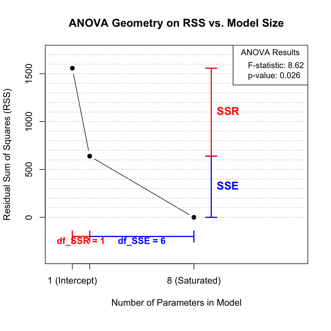

3.2.6 \(R^2\), \(F\) and a compact ANOVA table

Code

R2 <- SSR / SST; R2

[1] 0.5897229

Code

f  <- (SSR/1) / (SSE/(n-2)); f

[1] 8.624264

Code

pvf <- pf(f, df1 = 1, df2 = n-2, lower.tail = FALSE); pvf

[1] 0.0260588

Code

Ftable <- data.frame(
  Source = c("Regression", "Error"),
  df     = c(1, n - 2),
  SS     = c(SSR, SSE),
  MS     = c(SSR/1, SSE/(n-2)),
  F      = c(f, NA),
  pvalue = c(pvf, NA),
  R2part = c(SSR, SSE) / SST
)
Ftable

A call to anova() reproduces the same test:

Code

anova(fit.issu)

3.2.7 Sampling distributions via animation

Under \(H_0:\beta_1=0\), \(F\) follows \(F_{1,n-2}\). Under \(H_A\), the distribution shifts right (noncentral \(F\)).

3.2.7.1 Null world (\(H_0\) true)

Figure 3.1: Simulation under H0: animated GIF (HTML) and static PNG (PDF).

3.2.7.2 Alternative world (\(H_1\) true)

Figure 3.2: Simulation under HA (slope = -2): animated GIF for HTML, static PNG for PDF.

3.3 Example 2: Oxygen Purity Data

We model oxygen purity \(y\) as a function of hydrocarbon level \(x\) and report both mean response and prediction uncertainty.

3.3.1 Data

Code

x <- c(0.99, 1.02, 1.15, 1.29, 1.46, 1.36, 0.87, 1.23, 1.55, 1.40, 1.19,
       1.15, 0.98, 1.01, 1.11, 1.20, 1.26, 1.32, 1.43, 0.95)
y <- c(90.01, 89.05, 91.43, 93.74, 96.73, 94.45, 87.59, 91.77, 99.42, 93.65,
       93.54, 92.52, 90.56, 89.54, 89.85, 90.39, 93.25, 93.41, 94.98, 87.33)
n <- length(x); n

[1] 20

Code

purity.data <- data.frame(x = x, y = y)
head(purity.data)

3.3.2 Fit and quick summary

Code

fit <- lm(y ~ x, data = purity.data)
summary(fit)


Call:
lm(formula = y ~ x, data = purity.data)

Residuals:
     Min       1Q   Median       3Q      Max 
-1.83029 -0.73334  0.04497  0.69969  1.96809 

Coefficients:
            Estimate Std. Error t value Pr(>|t|)    
(Intercept)   74.283      1.593   46.62  < 2e-16 ***
x             14.947      1.317   11.35 1.23e-09 ***
---
Signif. codes:  0 '***' 0.001 '**' 0.01 '*' 0.05 '.' 0.1 ' ' 1

Residual standard error: 1.087 on 18 degrees of freedom
Multiple R-squared:  0.8774,    Adjusted R-squared:  0.8706 
F-statistic: 128.9 on 1 and 18 DF,  p-value: 1.227e-09

Interpretation. The slope’s sign gives the direction of association; its \(t\) test (or \(F\) with 1 df) assesses evidence for a trend. Look at \(\hat\sigma\) for noise scale and \(R^2\) for variance explained.

3.3.3 Scatter with fitted line

Code

plot(purity.data$x, purity.data$y,
     xlab = "Hydrocarbon level (x)", ylab = "Purity (y)",
     main = "Oxygen Purity vs Hydrocarbon Level")
abline(fit, col = "red", lwd = 2)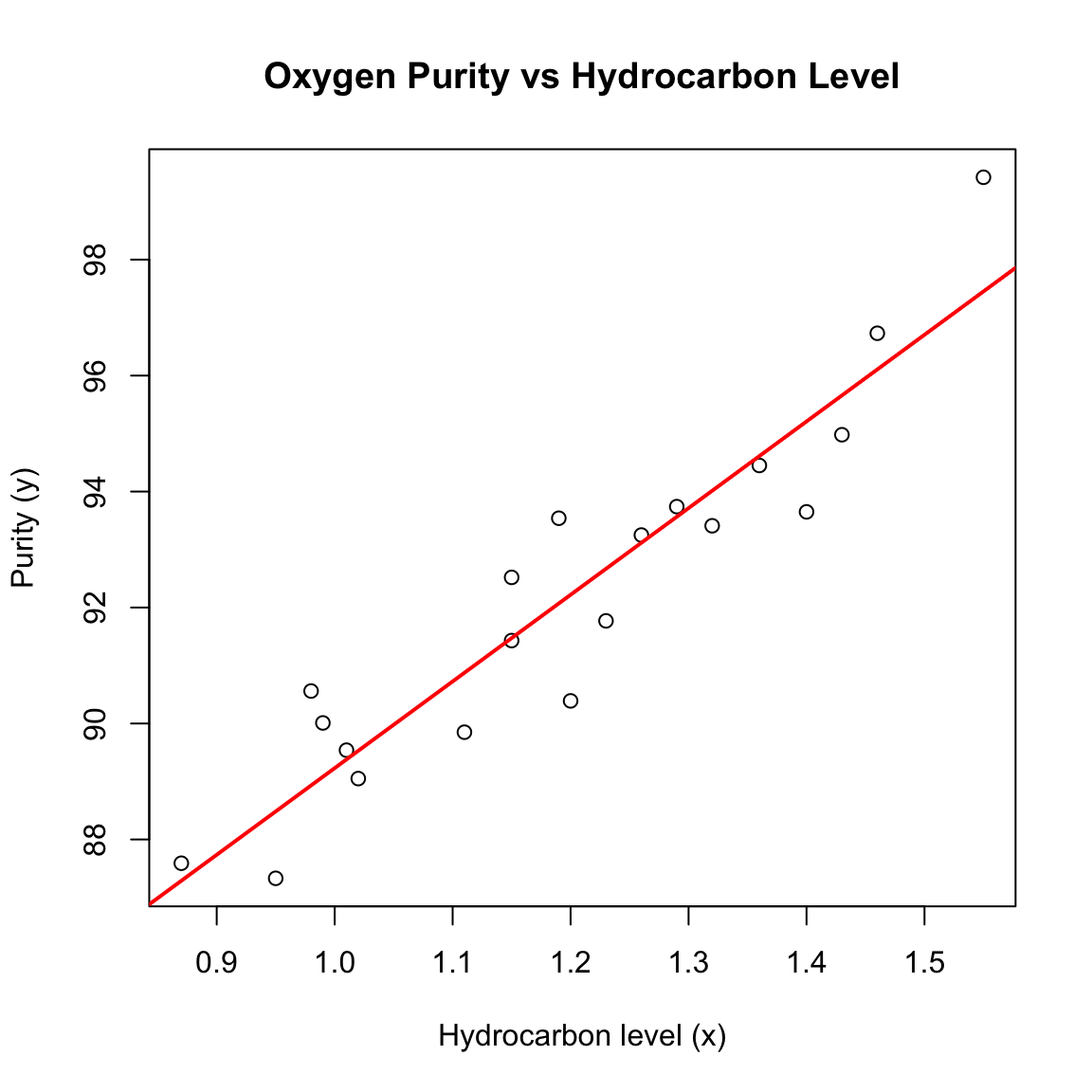

3.3.4 Coefficient CIs and ANOVA

Code

confint(fit, level = 0.95)

               2.5 %   97.5 %
(Intercept) 70.93555 77.63108
x           12.18107 17.71389

Code

anova(fit)

3.3.5 Mean-response and prediction bands

The mean-response CI narrows near \(\bar x\) and widens at the extremes; the prediction band is wider by the irreducible noise term.

Code

x0 <- seq(min(purity.data$x), max(purity.data$x), length = 50)
newdata <- data.frame(x = x0)

est.mean <- predict(fit, newdata = newdata, interval = "confidence", level = 0.95)
pred.new <- predict(fit, newdata = newdata, interval = "prediction", level = 0.95)

Code

plot(purity.data$x, purity.data$y,
     xlab = "Hydrocarbon level (x)", ylab = "Purity (y)",
     main = "Regression Line with Confidence and Prediction Bands")
abline(fit)
matlines(x0, est.mean[, 2:3], col = "blue", lty = 2, lwd = 2)
matlines(x0, pred.new[, 2:3], col = "red",  lty = 3, lwd = 2)
legend("topleft", c("Confidence Bands (mean)", "Prediction Bands (new y)"),
       col = c("blue", "red"), lty = 2:3, bty = "n")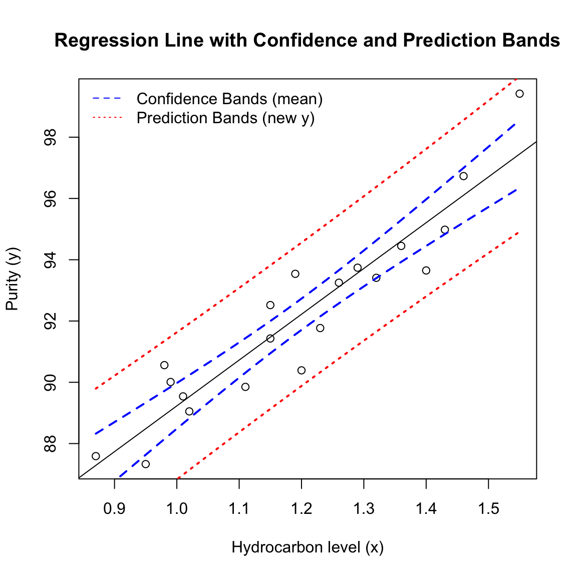

3.3.6 Residual diagnostics (assumptions check)

We look for no pattern in residuals vs. fits and approximate straightness in the Q–Q plot.

Code

pred <- fitted.values(fit)
e <- resid(fit)
d <- e / summary(fit)$sigma

par(mfrow = c(2,2))
plot(purity.data$x, purity.data$y, xlab = "x", ylab = "y"); abline(fit)
qqnorm(d, main = "Normal Q–Q"); qqline(d)
plot(pred, d, xlab = "Fitted", ylab = "Std. residuals", main = "Residuals vs Fits"); abline(h = 0, lty = 2)
plot(1:n, d, xlab = "Order", ylab = "Std. residuals", main = "Residuals vs Order"); abline(h = 0, lty = 2)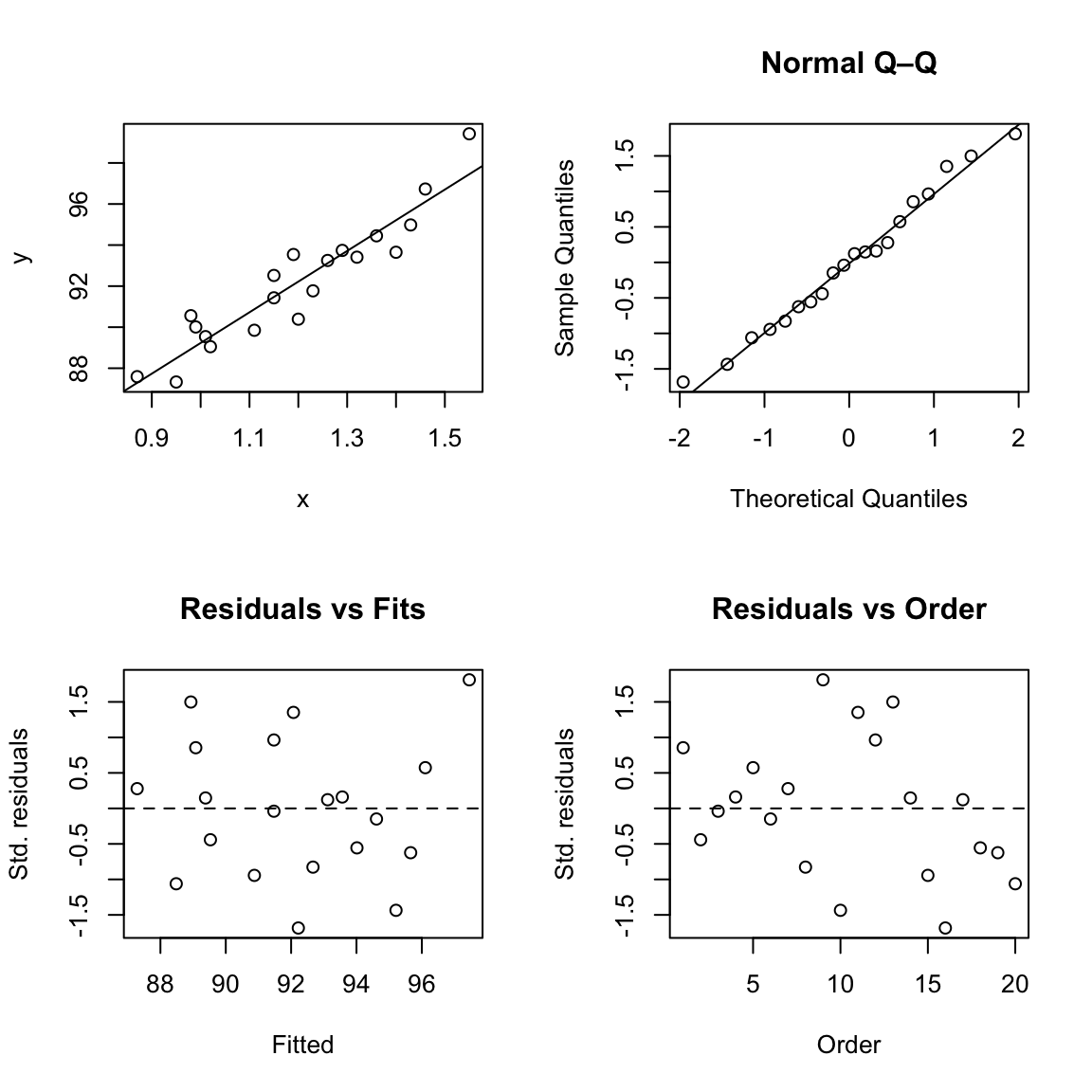

Code

par(mfrow = c(1,1))

3.4 Correlation analysis (for comparison, not causation)

Correlation summarizes linear association without fitting a line or making model assumptions.

3.4.1 Data and scatter

Code

strength <- c(9.95,24.45,31.75,35.00,25.02,16.86,14.38,9.60,24.35,
              27.50,17.08,37.00,41.95,11.66,21.65,17.89,69.00,10.30,
              34.93,46.59,44.88,54.12,56.63,22.13,21.15)
length <- c(2,8,11,10,8,4,2,2,9,8,4,11,12,2,4,4,20,1,10,
            15,15,16,17,6,5)
plot(length, strength, xlab = "Length", ylab = "Strength",
     main = "Strength vs Length (scatter)")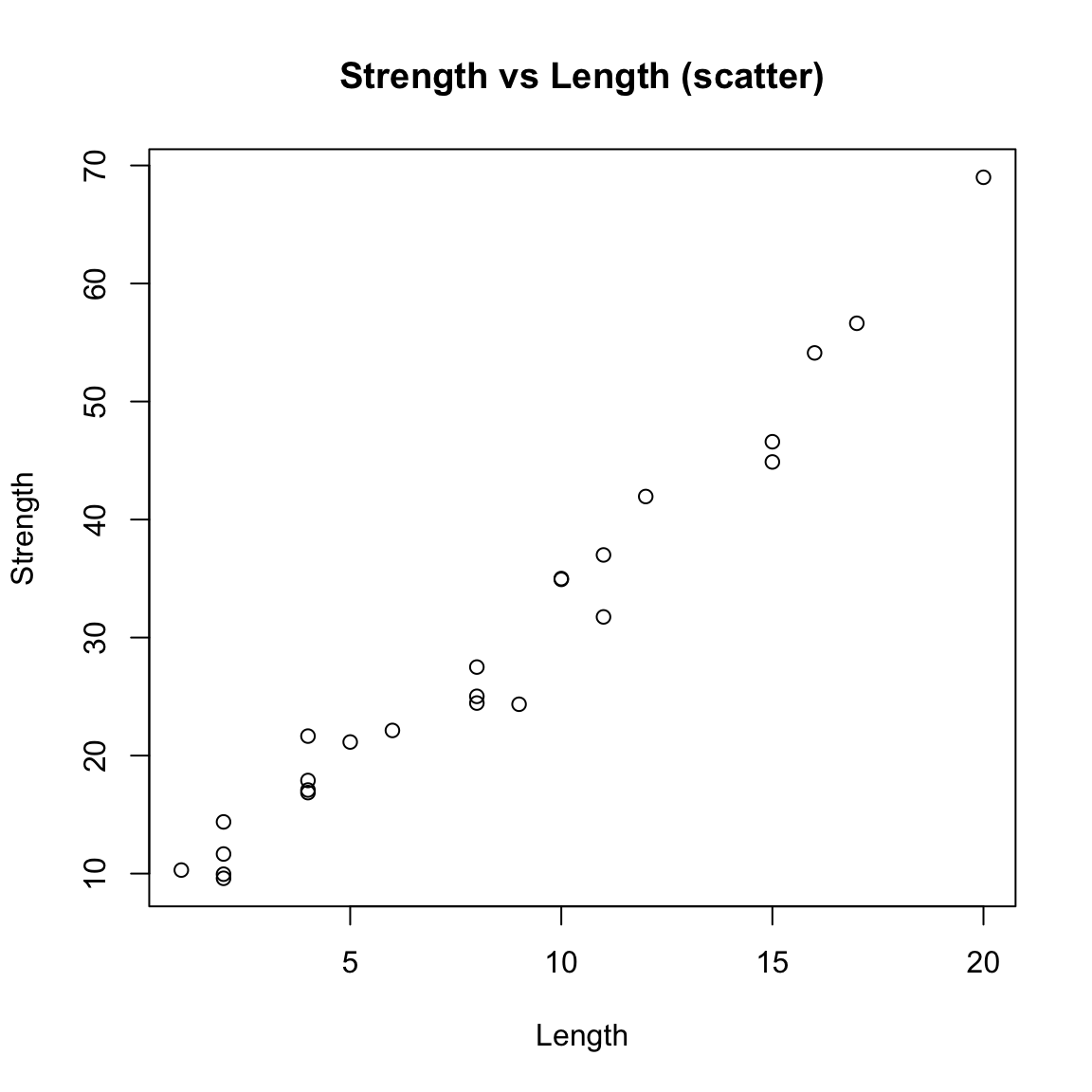

3.4.2 Pearson correlation and test

Code

cor(strength, length)

[1] 0.9818118

Code

cor.test(strength, length)


    Pearson's product-moment correlation

data:  strength and length
t = 24.801, df = 23, p-value < 2.2e-16
alternative hypothesis: true correlation is not equal to 0
95 percent confidence interval:
 0.9585414 0.9920735
sample estimates:
      cor 
0.9818118

Note. A large \(|r|\) and small \(p\) indicate linear association; regression further quantifies the slope and supports prediction, with diagnostics to check assumptions.

3.5 What to report (checklist)

Estimated line \(\hat y=\hat\beta_0+\hat\beta_1 x\) with units.
\(t\)/\(F\) test for slope, \(p\)-value and CI for \(\beta_1\).
\(R^2\) and \(\hat\sigma\) (RMSE) for fit quality.
Mean-response and prediction intervals at substantively relevant \(x_0\).
Residual diagnostics and any remedies (transformations, robust methods) if needed.