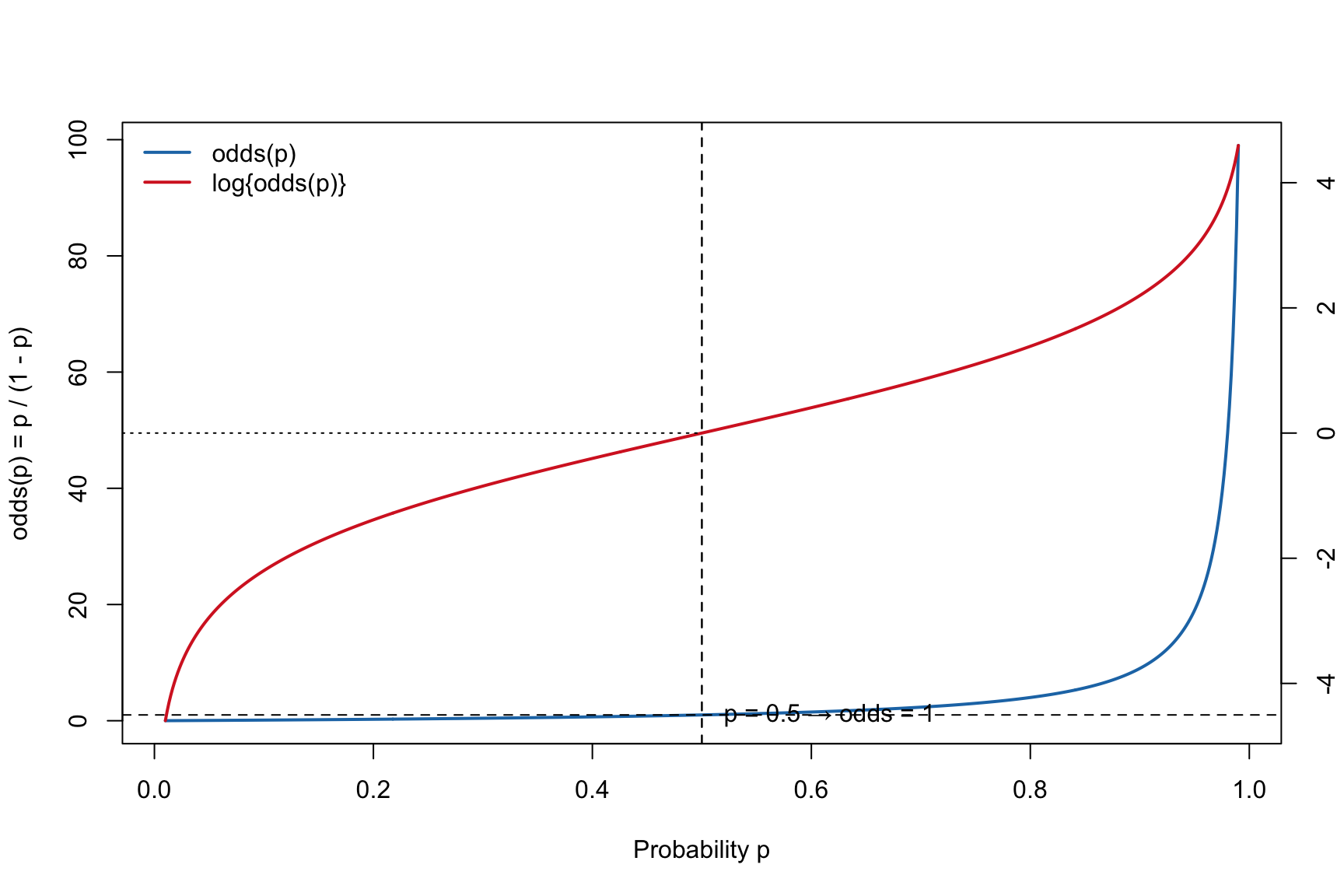
For an event with probability \(p\), the odds is \[\mathrm{odds}(p)=\frac{p}{1-p}\] and the log-odds (logit) is \[\mathrm{logit}(p)=\log\left(\frac{p}{1-p}\right)\].
Code
## Plot odds(p) with a right-hand axis for log(odds(p)),## using different line colors for the two curves.## Defaults: p in [0.01, 0.99].## Args:## p_min, p_max : endpoints for p-grid (0<p_min<p_max<1)## n : number of grid points## annotate : add reference lines/labels if TRUE## odds_col : color for odds(p)## logit_col : color for log(odds(p))## lwd1, lwd2 : line widths for the two curvesplot_odds <-function(p_min =0.01, p_max =0.99, n =400,annotate =TRUE,odds_col ="steelblue",logit_col ="firebrick",lwd1 =2, lwd2 =2) {stopifnot(p_min >0, p_max <1, p_min < p_max, n >=10) p <-seq(p_min, p_max, length.out = n) odds <- p / (1- p) logit <-log(odds)## Left y-axis: odds(p)plot(p, odds, type ="l", lwd = lwd1, col = odds_col,xlab ="Probability p",ylab ="odds(p) = p / (1 - p)")if (annotate) {abline(h =1, v =0.5, lty =2)text(0.52, 1.05, "p = 0.5 → odds = 1", adj =0) }## Right y-axis: logit(p) = log(odds) op <-par(new =TRUE)on.exit(par(op), add =TRUE)plot(p, logit, type ="l", lwd = lwd2, col = logit_col,axes =FALSE, xlab ="", ylab ="")axis(4)mtext("log{odds(p)} = log{p/(1 - p)}", side =4, line =3)if (annotate) {abline(v =0.5, lty =2)# logit(0.5) = 0 reference (horizontal) on the right-axis scale usr <-par("usr")segments(x0 = usr[1], y0 =0, x1 =0.5, y1 =0, lty =3) }legend("topleft",legend =c("odds(p)", "log{odds(p)}"),col =c(odds_col, logit_col),lwd =c(lwd1, lwd2), bty ="n")invisible(list(p = p, odds = odds, logit = logit))}## Example usage:## plot_odds() # defaults: steelblue for odds, firebrick for log-odds (right axis)plot_odds(odds_col ="#1f77b4", logit_col ="#d62728", n =600)
6.2 Logistic Regression
Let \(Y_i \in \{0,1\}\) denote a binary outcome, and let \(\mathbf{x}_i = (x_{i1}, \ldots, x_{ip})^\top\) be the vector of predictors excluding the intercept.
Let \(\boldsymbol{\beta} = (\beta_1, \ldots, \beta_p)^\top\) denote the slope coefficients, and \(\beta_0\) the intercept.
The logistic regression model specifies \[
p_i \;=\; P(Y_i = 1 \mid \mathbf{x}_i),
\] with \[
\log\!\left(\frac{p_i}{1 - p_i}\right)
\;=\; \beta_0 + \mathbf{x}_i^\top \boldsymbol{\beta}
\;=\; \beta_0 + \sum_{j=1}^p \beta_j x_{ij}.
\]
Equivalently, the fitted probability is \[
p_i(\mathbf{x}_i;\boldsymbol{\beta})
\;=\;
\frac{\exp(\beta_0 + \mathbf{x}_i^\top \boldsymbol{\beta})}
{1+\exp(\beta_0 + \mathbf{x}_i^\top \boldsymbol{\beta})}
\;=\;
\frac{1}{1+\exp\!\big(-(\beta_0 + \mathbf{x}_i^\top \boldsymbol{\beta})\big)}.
\]
This formulation expresses the log-odds of success as a linear function of predictors, ensuring that fitted probabilities remain in the range \((0,1)\).
The odds satisfy \[
\frac{p_i}{1-p_i} \;=\; \exp(\beta_0 + \mathbf{x}_i^\top \boldsymbol{\beta}),
\] so a one-unit increase in \(x_{ij}\) (holding other predictors fixed) multiplies the odds of success by \(\exp(\beta_j)\).
6.3 A Dataset Simulated from Logistic Regression
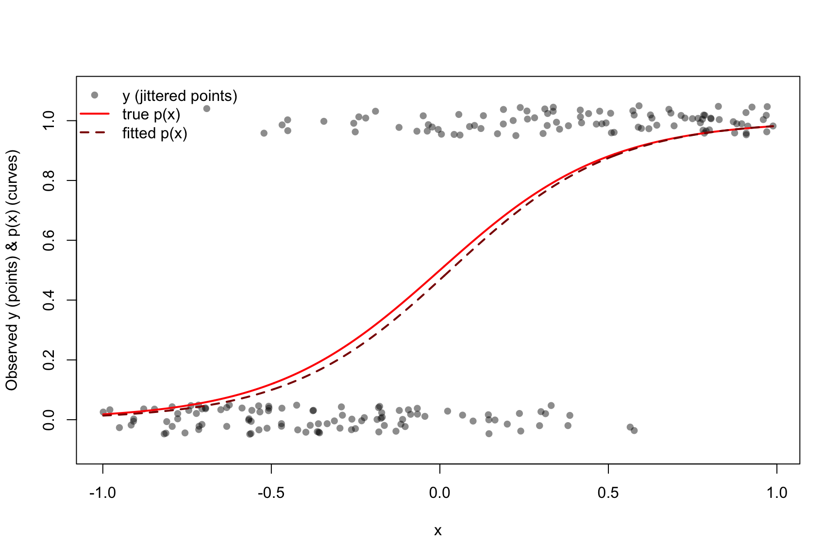
We simulate data from a logistic model where the logit is a linear function of \(x\):
We then display the observed \(y_i\) (binary outcomes) and the true probability curve \(p(x)\) in red.
Code
set.seed(123)## -- Truth (edit as desired) --n <-200beta0 <-0beta1 <-4## -- Simulate --x <-runif(n, -1, 1) # predictoreta <- beta0 + beta1 * xp <-plogis(eta) # true p(x)y <-rbinom(n, size =1, prob = p) # outcomessim.data <-data.frame(x = x, y = y, p = p)
6.3.1 Fit a logistic model to the simulated data
Code
## -- Optional: fit a model to the simulated data --sim.fit <-glm(y ~ x, data = sim.data, family =binomial())p_fit <-predict(sim.fit, newdata =data.frame(x = x), type ="response")## -- Plot: points for y_i (jittered), red line for true p(x) --## Define jitter amountjit <-0.05## jitter to separate 0/1 visuallyyj <-jitter(sim.data$y, amount = jit) plot(sim.data$x, yj,pch =16, col =rgb(0, 0, 0, 0.45),xlab ="x",ylab ="Observed y (points) & p(x) (curves)",ylim =c(-0.1, 1.1))## True probability curve (red)xg <-seq(min(x), max(x), length.out =500)lines(xg, plogis(beta0 + beta1 * xg), col ="red", lwd =2)## Optional: add fitted probability curve (dashed dark red)lines(xg, predict(sim.fit, newdata =data.frame(x = xg), type ="response"),col ="darkred", lwd =2, lty =2)legend("topleft",legend =c("y (jittered points)", "true p(x)", "fitted p(x)"),pch =c(16, NA, NA),lty =c(NA, 1, 2),col =c(rgb(0,0,0,0.45), "red", "darkred"),lwd =c(NA, 2, 2),bty ="n")
6.4 Example: Coronary Heart Disease Data
6.4.1 Load a dataset
This dataset is about a follow-up study to determine the development of coronary heart disease (CHD) over 9 years of follow-up of 609 white males from Evans County, Georgia.
Variable meanings (as provided):
chd: 1 if a person has the disease, 0 otherwise.
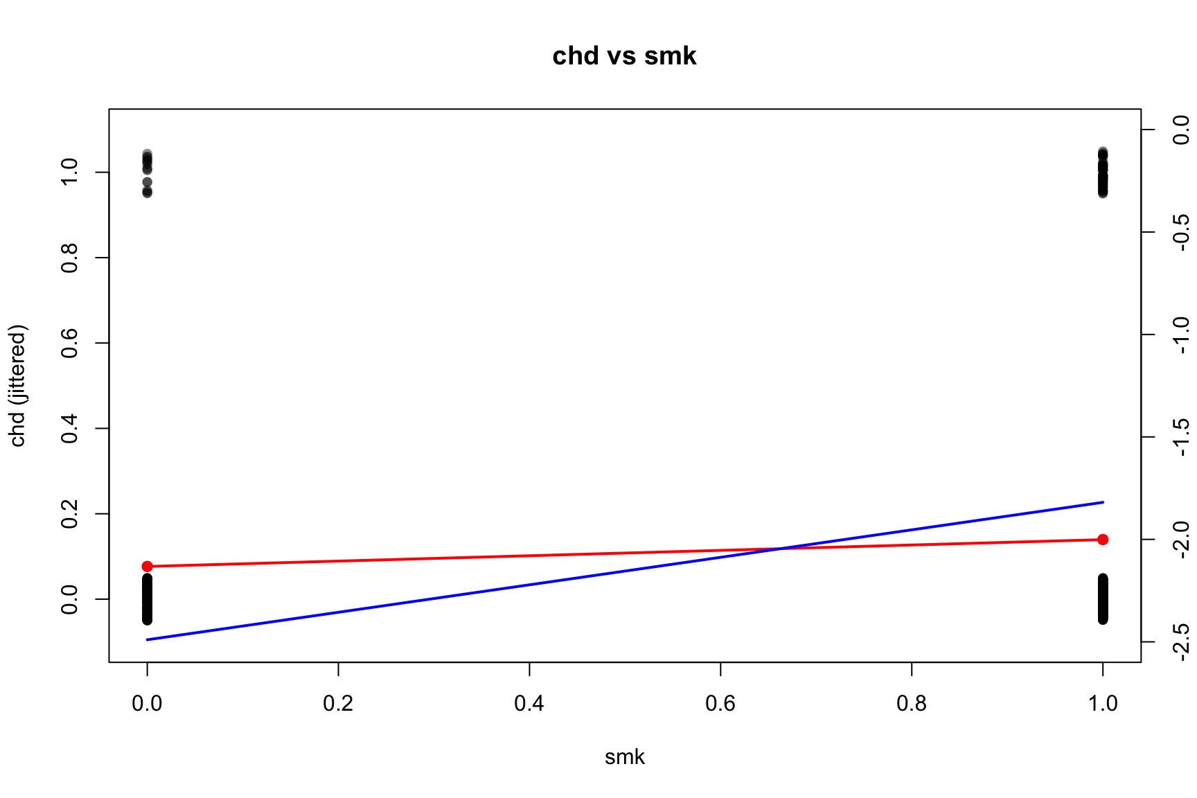
smk: 1 if smoker, 0 if not.
cat: 1 if catecholamine level is high, 0 if low.
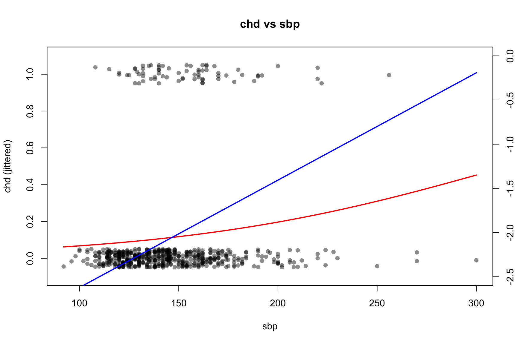
sbp: systolic blood pressure (continuous).
age: age in years (continuous).
chl: cholesterol level (continuous).
ecg: 1 if electrocardiogram is abnormal, 0 if normal.
hpt: 1 if high blood pressure, 0 if normal.
Code
## Adjust the path if needed. The default is your original V: drive path.data_path <-"evans.dat"## Read data (expects a header row)CHD.data <-read.table(data_path, header =TRUE)if (knitr::is_html_output()){ CHD.data} else{ CHD.data[1:20,]}
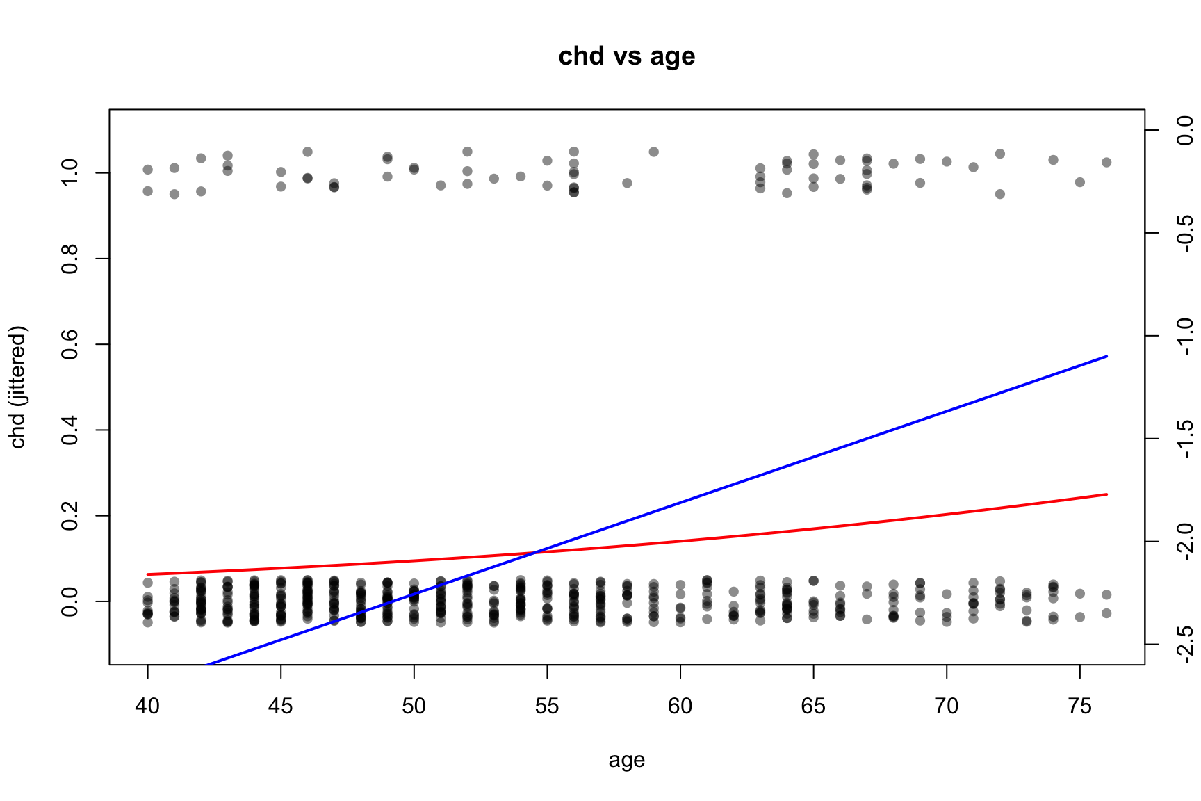
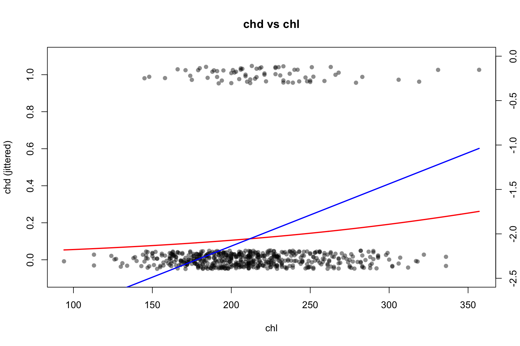
6.4.2 Fit Logistic Regression Model for a Single Variable
Code
vars <-c("smk", "sbp", "age", "chl")#jit <- 0.01 # global jitter amount for y## par(mfrow = c(2, 2), mar = c(4, 4, 2, 4) + 0.1) # extra right margin for axis(4)for (v in vars) {## Univariate logistic regression using ORIGINAL variable name in the formula fit <-glm(formula =reformulate(v, response ="chd"),data = CHD.data,family =binomial() )print(summary(fit))## Base scatter of chd with small jitter (left axis: probability scale)plot( CHD.data[[v]],jitter(CHD.data$chd, amount = jit),pch =16, col =rgb(0, 0, 0, 0.45),xlab = v, ylab ="chd (jittered)",main =paste("chd vs", v),ylim =c(-0.1, 1.1) )## Fitted π(x) in red (left axis)if (length(unique(CHD.data[[v]])) ==2) {# binary predictor xcat <-sort(unique(CHD.data[[v]])) nd <-setNames(data.frame(xcat), v) pcat <-predict(fit, newdata = nd, type ="response")points(xcat, pcat, pch =19, col ="red")lines(xcat, pcat, col ="red", lwd =2)# Right-axis: logit{π(x)} with fixed y-limits logit_p <-log(pcat / (1- pcat))par(new =TRUE)plot( xcat, logit_p, type ="l", lwd =2, col ="blue",axes =FALSE, xlab ="", ylab ="",xlim =range(CHD.data[[v]]), ylim =c(-2.5, 0) )axis(4)mtext("logit(p(x))", side =4, line =3)par(new =FALSE) } else {# continuous predictor xg <-seq(min(CHD.data[[v]]), max(CHD.data[[v]]), length.out =400) nd <-setNames(data.frame(xg), v) pg <-predict(fit, newdata = nd, type ="response")lines(xg, pg, col ="red", lwd =2)# Right-axis: logit{π(x)} with fixed y-limits logit_pg <-log(pg / (1- pg))par(new =TRUE)plot( xg, logit_pg, type ="l", lwd =2, col ="blue",axes =FALSE, xlab ="", ylab ="",xlim =range(xg), ylim =c(-2.5, 0) )axis(4)mtext("logit(p(x))", side =4, line =3)par(new =FALSE) }}
Call:
glm(formula = reformulate(v, response = "chd"), family = binomial(),
    data = CHD.data)

Coefficients:
            Estimate Std. Error z value Pr(>|z|)
(Intercept)  -2.4898     0.2524  -9.865   <2e-16 ***
smk           0.6706     0.2919   2.297   0.0216 *
---
Signif. codes:  0 '***' 0.001 '**' 0.01 '*' 0.05 '.' 0.1 ' ' 1

(Dispersion parameter for binomial family taken to be 1)

    Null deviance: 438.56  on 608  degrees of freedom
Residual deviance: 432.81  on 607  degrees of freedom
AIC: 436.81

Number of Fisher Scoring iterations: 5
Call:
glm(formula = reformulate(v, response = "chd"), family = binomial(),
    data = CHD.data)

Coefficients:
             Estimate Std. Error z value Pr(>|z|)
(Intercept) -3.837912   0.629805  -6.094  1.1e-09 ***
sbp          0.012154   0.004036   3.011   0.0026 **
---
Signif. codes:  0 '***' 0.001 '**' 0.01 '*' 0.05 '.' 0.1 ' ' 1

(Dispersion parameter for binomial family taken to be 1)

    Null deviance: 438.56  on 608  degrees of freedom
Residual deviance: 430.06  on 607  degrees of freedom
AIC: 434.06

Number of Fisher Scoring iterations: 4
Call:
glm(formula = reformulate(v, response = "chd"), family = binomial(),
    data = CHD.data)

Coefficients:
            Estimate Std. Error z value Pr(>|z|)
(Intercept) -4.47833    0.75610  -5.923 3.16e-09 ***
age          0.04445    0.01315   3.381 0.000723 ***
---
Signif. codes:  0 '***' 0.001 '**' 0.01 '*' 0.05 '.' 0.1 ' ' 1

(Dispersion parameter for binomial family taken to be 1)

    Null deviance: 438.56  on 608  degrees of freedom
Residual deviance: 427.22  on 607  degrees of freedom
AIC: 431.22

Number of Fisher Scoring iterations: 5
Call:
glm(formula = reformulate(v, response = "chd"), family = binomial(),
    data = CHD.data)

Coefficients:
             Estimate Std. Error z value Pr(>|z|)
(Intercept) -3.538260   0.686879  -5.151 2.59e-07 ***
chl          0.007004   0.003064   2.286   0.0223 *
---
Signif. codes:  0 '***' 0.001 '**' 0.01 '*' 0.05 '.' 0.1 ' ' 1

(Dispersion parameter for binomial family taken to be 1)

    Null deviance: 438.56  on 608  degrees of freedom
Residual deviance: 433.42  on 607  degrees of freedom
AIC: 437.42

Number of Fisher Scoring iterations: 4
6.4.3 Fit Logistic Regression Model with all variables
Call:
glm(formula = chd ~ smk + cat + sbp + age + chl + ecg + hpt,
    family = binomial(link = "logit"), data = CHD.data)

Coefficients:
             Estimate Std. Error z value Pr(>|z|)
(Intercept) -6.048892   1.345165  -4.497  6.9e-06 ***
smk          0.855951   0.306505   2.793  0.00523 **
cat          0.732763   0.376129   1.948  0.05139 .
sbp         -0.006995   0.006976  -1.003  0.31600
age          0.033956   0.015344   2.213  0.02690 *
chl          0.008970   0.003274   2.740  0.00615 **
ecg          0.417776   0.295553   1.414  0.15750
hpt          0.655498   0.359976   1.821  0.06861 .
---
Signif. codes:  0 '***' 0.001 '**' 0.01 '*' 0.05 '.' 0.1 ' ' 1

(Dispersion parameter for binomial family taken to be 1)

    Null deviance: 438.56  on 608  degrees of freedom
Residual deviance: 399.35  on 601  degrees of freedom
AIC: 415.35

Number of Fisher Scoring iterations: 5
Notes for interpretation:
Positive coefficients increase the log-odds of CHD; negative coefficients decrease it.
For indicator variables (e.g., smk), exp(beta) is the adjusted odds ratio comparing the group with value 1 versus 0, holding others fixed.
For continuous predictors (e.g., sbp, age), exp(beta) is the multiplicative change in the odds for a one‑unit increase. For a d-unit increase, the OR is exp(d * beta).
6.5 Inference for Coefficients: Confidence Intervals and Covariance Matrix
We extract profile‑likelihood CIs and the covariance matrix to confirm standard errors.
Code
ci_95 <-confint(fit1_chd, level =0.95) # profile-likelihood CIvcov_mat <-vcov(fit1_chd) # covariance matrix of coefficientsse_vec <-sqrt(diag(vcov_mat)) # standard errorsci_95
The or_from_predict R function is a utility designed to calculate the Odds Ratio (OR) and its 95% confidence interval (CI) between two specific covariate profiles (new1 and new0) for a given logistic regression model (fit). The calculation is performed on the link (logit) scale. For a logistic model \(\text{logit}(p) = \eta = \mathbf{X}\boldsymbol{\beta}\), the log-Odds Ratio (logOR) is the difference between the linear predictors (\(\eta_1, \eta_0\)) for the two profiles: \[\widehat{\text{logOR}} = \eta_1 - \eta_0 = (\mathbf{x}_1^T - \mathbf{x}_0^T) \boldsymbol{\beta} = \mathbf{c}^T \boldsymbol{\beta} \tag{6.1}\]
Here, \(\mathbf{c} = \mathbf{x}_1 - \mathbf{x}_0\) is the linear contrast vector derived from the model matrices of the two profiles. The function estimates the variance of this contrast as \(\text{Var}(\widehat{\text{logOR}}) = \mathbf{c}^T \mathbf{V} \mathbf{c}\), where \(\mathbf{V}\) is the model’s variance-covariance matrix (vcov(fit)). The standard error \(SE = \sqrt{\mathbf{c}^T \mathbf{V} \mathbf{c}}\) is used to compute the \(100(1-\alpha)\%\) confidence interval for the logOR: \[\widehat{\text{logOR}} \pm z_{1-\alpha/2} \times SE.\] These values (estimate and CI bounds) are then exponentiated to produce the final \(\widehat{\text{OR}} = \exp(\widehat{\text{logOR}})\) and its 95% CI. The function also prints two helpful summaries to the console: a data frame showing only the variables that differ between the new0 and new1 profiles, and a 2x3 table presenting the estimates and CIs for both the OR and the logOR.
The R function to find ORs
Code
## Compute OR and 95% CI via predict() on the LINK scale## OR = exp( eta(new1) - eta(new0) ), where eta(.) = logit{π(.)}## Compute OR via predict() contrast on the LINK scale, also:## (ii) print a 2-row data.frame of only variables that differ between new0 and new1## (iii) print a 2x3 table (rows: OR, logOR; cols: Estimate, CI_low, CI_up)or_from_predict <-function(fit, new1, new0, level =0.95, digits =4, tol =1e-12) {stopifnot(is.data.frame(new1), is.data.frame(new0))## --- REFACTORED SECTION START ---## ---- (ii) Two-row data.frame with only changed variables ----## Helper function to find differing variables between two profiles## This is defined *inside* or_from_predict for encapsulation get_changed_vars <-function(d0, d1, tolerance) { common <-intersect(names(d0), names(d1)) diffv <-vapply(common, function(nm) { x0 <- d0[[nm]]; x1 <- d1[[nm]]if (is.numeric(x0) &&is.numeric(x1)) {!isTRUE(all.equal(as.numeric(x0), as.numeric(x1), tolerance = tolerance)) } else {!identical(x0, x1) } }, logical(1)) keep <- common[diffv]if (length(keep) ==0L) { out <-data.frame(`_no_changes_`="no differences")rownames(out) <-c("new0", "new1")return(out) } out <-rbind(d0[keep], d1[keep])rownames(out) <-c("new0", "new1") out }## Call the helper function changes_df <-get_changed_vars(new0, new1, tol)## --- REFACTORED SECTION END ---## ---- Linear contrast for log-OR and its variance ----## (i) Calculate logOR estimate using predict(type="link")## eta(.) = logit{p(.)} eta1 <-predict(fit, newdata = new1, type ="link") eta0 <-predict(fit, newdata = new0, type ="link") logOR_hat <-as.numeric(eta1 - eta0) # logOR = eta1 - eta0## (ii) Calculate standard error using the contrast vector 'cvec' X1 <-model.matrix(delete.response(terms(fit)), data = new1) X0 <-model.matrix(delete.response(terms(fit)), data = new0) cvec <-as.numeric(X1 - X0) V <-vcov(fit) se_logOR <-sqrt(as.numeric(t(cvec) %*% V %*% cvec)) alpha <-1- level z <-qnorm(1- alpha /2) ci_log <-c(logOR_hat - z * se_logOR, logOR_hat + z * se_logOR)## ---- 2x3 table: rows OR and logOR; columns Estimate, CI_low, CI_up ---- res_tab <-data.frame(Estimate =c(exp(logOR_hat), logOR_hat),CI_low =c(exp(ci_log[1L]), ci_log[1L]),CI_up =c(exp(ci_log[2L]), ci_log[2L]),row.names =c("OR", "logOR") )## ---- Print requested items ----cat("\nVariables that differ between new0 and new1:\n")print(changes_df)cat("\nOdds Ratio summary:\n")print(round(res_tab, digits = digits)) # Added rounding for neatness## ---- Return (invisibly) ----invisible(list(OR =exp(logOR_hat),CI_OR =exp(ci_log),logOR = logOR_hat,CI_logOR = ci_log,se_logOR = se_logOR,changes = changes_df,table = res_tab ))}## --- Example usage ---## Suppose 'fit1_chd' is your fitted model and 'CHD.data' is your data## base_prof <- as.data.frame(lapply(CHD.data, function(col) if (is.numeric(col)) mean(col) else col[1]))## new0 <- base_prof; new0$smk <- 0## new1 <- base_prof; new1$smk <- 1## or_from_predict(fit1_chd, new1 = new1, new0 = new0)mean_profile <-function(data, vars_binary_as =c(0,1)) {## Build a single-row data.frame of typical values: out <-lapply(data, function(col) {if (is.numeric(col)) {# If strictly 0/1, keep mean (works fine for GLM prediction),# or switch to mode if you prefer.if (all(col %in%c(0,1))) mean(col) elsemean(col, na.rm =TRUE) } else {# Fallback to first level for factors/charactersif (is.factor(col)) levels(col)[1] elseunique(col)[1] } })as.data.frame(out)}
6.6.2 Examples of Finding ORs and Their CIs for the CHD Dataset
6.6.2.1 OR Smoking (smk) (1 vs 0)
Code
### 1) Smoking OR: smk = 1 vs 0 (other vars at their means)## Example profiles at sample means (adjust as you like)base_prof <-mean_profile(CHD.data)new0 <- base_prof; new0$smk <-0new1 <- base_prof; new1$smk <-1res_smk <-or_from_predict(fit1_chd, new1 = new1, new0 = new0)
Variables that differ between new0 and new1:
     smk
new0   0
new1   1

Odds Ratio summary:
      Estimate CI_low  CI_up
OR      2.3536 1.2907 4.2917
logOR   0.8560 0.2552 1.4567
How to read this:
OR_smk > 1 suggests higher odds of CHD among smokers (adjusted for other variables). If the 95% CI excludes 1, the association is statistically significant at the 5% level.
6.6.2.2 OR for Systolic Blood Pressure (sbp): from 120 to 160
We compute the adjusted OR for a 40‑unit increase in sbp (from 120 to 160):
Code
### 2) SBP OR: 160 vs 120 (other vars at their means)new0 <- base_prof; new0$sbp <-120new1 <- base_prof; new1$sbp <-160res_sbp <-or_from_predict(fit1_chd, new1 = new1, new0 = new0)
Variables that differ between new0 and new1:
     sbp
new0 120
new1 160

Odds Ratio summary:
      Estimate  CI_low  CI_up
OR      0.7559  0.4375 1.3062
logOR  -0.2798 -0.8267 0.2671
6.6.2.3 OR for Combined Effects of Two Variables: Smoking with an Age Difference
Suppose we compare two groups that differ in smoking status and age:
Group A:smk = 1, age = 50 (all other covariates equal)
Group B:smk = 0, age = 30
The log‑odds contrast is (\(A = \beta_{smk} + (50-20)\beta_{age}\)), so the OR is (\(\exp(A)\)).
Variables that differ between new0 and new1:
     age smk
new0  30   0
new1  50   1

Odds Ratio summary:
      Estimate CI_low   CI_up
OR      4.6417 1.8546 11.6168
logOR   1.5351 0.6177  2.4525
6.7 Assessing Statistical Significance with Wilks’ Theorem (Analogue of F-test for OLS)
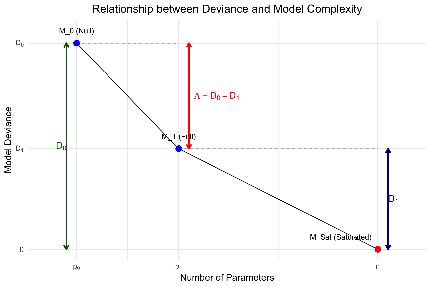
In the context of logistic regression, Wilks’ theorem provides the basis for the Likelihood Ratio Test (LRT) used to assess the significance of predictor variables. The theorem states that when comparing a full model (\(M_1\)) to a nested null model (\(M_0\)), the test statistic, \(\Lambda\), asymptotically follows a chi-squared (\(\chi^2\)) distribution under the null hypothesis (i.e., that the simpler model \(M_0\) is correct).
The statistic \(\Lambda\) is calculated as the difference in the maximized log-likelihoods: \[\Lambda = -2(\log L_0 - \log L_1) \tag{6.2}\] where \(\log L_0\) and \(\log L_1\) are the log-likelihoods of the null and full models, respectively. In logistic regression, this is equivalent to the difference in the deviances: \(\Lambda = \text{Deviance}_0 - \text{Deviance}_1\). This test statistic \(\Lambda\) represents the reduction in deviance (a measure of badness-of-fit) achieved by adding the extra predictors to the model.
The following R code chunk generates a conceptual plot of this relationship:
Code
#| label: plot-lrt-concept#| echo: false#| fig-cap: "Conceptual plot of Deviance versus Number of Parameters, illustrating the Likelihood Ratio Test statistic (Λ) and Residual Deviance. Λ is the drop from the Null Model to the Full Model. The Saturated Model represents perfect fit (Deviance = 0)."library(ggplot2)## 1. Create conceptual data for the plot## These are just for illustrationn_obs <-60# Number of observationsp0 <-1# Parameters in null model (intercept)p1 <-21# Parameters in full model (e.g., intercept + 7 predictors)psat <- n_obs # Parameters in saturated model (1 per observation)D0 <-41# Null devianceD1 <-20# Full model deviance (residual deviance of M1)D_sat <-0# Saturated model deviance## Data frame for the three pointsplot_data <-data.frame(model =c("M_0 (Null)", "M_1 (Full)", "M_Sat (Saturated)"),params =c(p0, p1, psat),deviance =c(D0, D1, D_sat),## Add custom justification and nudges for labelshjust_val =c(0.5, 0.5, 1.1), # Right-align the last labelnudge_x_val =c(0, 0, 0) )## 2. Create the ggplotggplot(plot_data, aes(x = params, y = deviance)) +## Draw dashed guide lines for D0 and D1geom_segment(aes(x = p0, y = D0, xend = p1, yend = D0), linetype ="dashed", color ="grey70") +geom_segment(aes(x = p1, y = D1, xend = psat, yend = D1), linetype ="dashed", color ="grey70") +## Connect the points with linesgeom_line(color ="black", linetype ="solid", linewidth =0.5) +## Draw the main pointsgeom_point(size =4, aes(color = model)) +## --- MODIFIED LABEL PLACEMENT ---## Label the points using custom nudge/justificationgeom_text(aes(label = model, hjust = hjust_val, nudge_x = nudge_x_val), nudge_y =2.5, # Use a much smaller vertical nudgesize =4 ) +## --- ADDED BACK D0 and D1 ANNOTATIONS ---## D0 (Null Deviance)geom_segment(aes(x = p0 -2, y = D0, xend = p0 -2, yend = D_sat), # Nudged leftarrow =arrow(ends ="both", length =unit(0.1, "inches")),color ="darkgreen",linewidth =1 ) +annotate("text",x = p0 -3, y = D0 /2, # Nudged leftlabel ="D[0]", parse =TRUE,color ="darkgreen", hjust =0.5, size =5 ) +## D1 (Residual Deviance of Full Model)geom_segment(aes(x = psat +2, y = D1, xend = psat +2, yend = D_sat), # Nudged rightarrow =arrow(ends ="both", length =unit(0.1, "inches")),color ="darkblue",linewidth =1 ) +annotate("text",x = psat +3, y = D1 /2, # Nudged rightlabel ="D[1]", parse =TRUE,color ="darkblue", hjust =0.5, size =5 ) +## LRT statistic Λ = D0 - D1geom_segment(aes(x = p1 +2, y = D0, xend = p1 +2, yend = D1), # Nudged rightarrow =arrow(ends ="both", length =unit(0.1, "inches")),color ="red",linewidth =1 ) +annotate("text",x = p1 +3, y = D1 + (D0 - D1) /2, # Nudged rightlabel ="Lambda == D[0] - D[1]",parse =TRUE,color ="red", hjust =0, size =5 ) +## Customize axes to show the symbolic labelsscale_x_continuous(breaks =c(p0, p1, psat),labels =c(expression(p[0]), expression(p[1]), expression(n)),expand =expansion(mult =0.1) # Add some padding ) +scale_y_continuous(breaks =c(D_sat, D1, D0),labels =c(expression(0), expression(D[1]), expression(D[0])) ) +## Labels and Titlelabs(title ="Relationship between Deviance and Model Complexity",x ="Number of Parameters",y ="Model Deviance" ) +## Clean themetheme_minimal(base_size =14) +theme(plot.title =element_text(hjust =0.5),legend.position ="none"# Remove legend, as points are labeled ) +scale_color_manual(values =c("M_0 (Null)"="blue", "M_1 (Full)"="blue", "M_Sat (Saturated)"="red"))
As the diagram illustrates, the null model (\(M_0\)) has fewer parameters (\(p_0\)) and a higher deviance (\(D_0\), or worse fit), while the full model (\(M_1\)) has more parameters (\(p_1\)) and a lower deviance (\(D_1\)). The Likelihood Ratio Test statistic \(D\) is the magnitude of this drop in deviance.
For assessing the overall significance of a regression model (fit1_chd), this involves comparing it to its corresponding intercept-only (null) model. The degrees of freedom for the \(\chi^2\) test is the difference in the number of parameters, \(df = p_1 - p_0\), which equals the number of predictors in the full model.
Here is an R code chunk demonstrating how to compute this p-value directly from a glm fit object, assuming it is named fit1_chd.
Code
## Calculate the Likelihood Ratio Test statistic (D) and degrees of freedom (df)## by comparing the model's deviance to the null (intercept-only) deviance,## both of which are stored in the 'fit1_chd' object.summary(fit1_chd)
Call:
glm(formula = chd ~ smk + cat + sbp + age + chl + ecg + hpt,
    family = binomial(link = "logit"), data = CHD.data)

Coefficients:
             Estimate Std. Error z value Pr(>|z|)
(Intercept) -6.048892   1.345165  -4.497  6.9e-06 ***
smk          0.855951   0.306505   2.793  0.00523 **
cat          0.732763   0.376129   1.948  0.05139 .
sbp         -0.006995   0.006976  -1.003  0.31600
age          0.033956   0.015344   2.213  0.02690 *
chl          0.008970   0.003274   2.740  0.00615 **
ecg          0.417776   0.295553   1.414  0.15750
hpt          0.655498   0.359976   1.821  0.06861 .
---
Signif. codes:  0 '***' 0.001 '**' 0.01 '*' 0.05 '.' 0.1 ' ' 1

(Dispersion parameter for binomial family taken to be 1)

    Null deviance: 438.56  on 608  degrees of freedom
Residual deviance: 399.35  on 601  degrees of freedom
AIC: 415.35

Number of Fisher Scoring iterations: 5
Code
lrt_statistic <- fit1_chd$null.deviance - fit1_chd$deviancelrt_df <- fit1_chd$df.null - fit1_chd$df.residual## Compute the p-value from the chi-squared distribution## We use lower.tail = FALSE to get P(ChiSq > D)p_value <-pchisq(lrt_statistic, lrt_df, lower.tail =FALSE)## Create and print the result in an ANOVA-like table## Row 1: Null model## Row 2: Full model (fit1_chd), showing the test against the nulllrt_table <-data.frame("Resid. Df"=c(fit1_chd$df.null, fit1_chd$df.residual),"Resid. Dev"=c(round(fit1_chd$null.deviance, 4), round(fit1_chd$deviance, 4)),"Test Df"=c(NA, lrt_df),"Test Statistic (D)"=c(NA, round(lrt_statistic, 4)),"p-value"=c(NA, format.pval(p_value, digits =4)),row.names =c("Null Model", "Full Model (fit1_chd)"),check.names =FALSE# Prevent R from changing 'p-value' to 'p.value')cat("Likelihood Ratio Test for Model Significance:\n")
Likelihood Ratio Test for Model Significance:
Code
lrt_table
Using built-in anova() function
Code
fit0_chd <-glm (chd~1, data = CHD.data, family =binomial())anova(fit0_chd, fit1_chd)
Code
anova(fit1_chd, test="LRT")
6.8 Assessing Predictive Effect-Size (Anologue to \(R^2_\mathrm{adj}\))
While the LRT assesses overall model significance (in-sample fit), it’s also crucial to evaluate how well the model predicts new, unseen data (out-of-sample performance). A common method is to split the data into a training set (e.g., 2/3 of the data) and a test set (e.g., 1/3). The model is fit using only the training data and then used to make predictions for the test data. We can then compare these predictions to the actual outcomes in the test set.
6.8.1 Understanding the Confusion Matrix and Metrics
To evaluate a model’s predictive performance, we classify its probabilistic predictions using a threshold (typically 0.5) and compare them to the true outcomes in a Confusion Matrix:
Predicted: 0
Predicted: 1
Actual: 0
True Negative (TN)
False Positive (FP)
Actual: 1
False Negative (FN)
True Positive (TP)
From this matrix, we derive several key performance metrics:
Misclassification Error Rate (ER): The proportion of all predictions that were incorrect. \[
\text{Error Rate} = \frac{FP + FN}{TP + TN + FP + FN}
\]
Precision (Positive Predictive Value): Answers: “Of all the times the model predicted positive, how often was it correct?” This is crucial when the cost of a False Positive is high. \[
\text{Precision} = \frac{TP}{TP + FP}
\]
Recall (Sensitivity or True Positive Rate): Answers: “Of all the actual positive cases, how many did the model find?” This is crucial when the cost of a False Negative is high. \[
\text{Recall (TPR)} = \frac{TP}{TP + FN}
\]
ROC Curve and AUC: An ROC (Receiver Operating Characteristic) Curve is a graph that shows a model’s diagnostic ability across all possible classification thresholds. It plots the True Positive Rate (Recall) on the y-axis against the False Positive Rate (FPR = \(\frac{FP}{FP + TN}\)) on the x-axis.
Interpretation: The curve shows the trade-off between sensitivity (finding all the positives) and specificity (not mislabeling negatives). A random “no-skill” classifier is represented by a diagonal line from (0,0) to (1,1). A perfect classifier would hug the top-left corner (TPR = 1, FPR = 0).
AUC (Area Under the Curve): The AUC summarizes the entire curve into a single number from 0 to 1. An AUC of 0.5 corresponds to a random guess, while an AUC of 1.0 represents a perfect model.
Precision-Recall (PR) Curve: A PR Curve plots Precision (y-axis) against Recall (x-axis) at all possible thresholds.
Interpretation: This curve shows the trade-off between how reliable a positive prediction is (Precision) and how complete the model is at finding all positives (Recall).
When to Use: The PR curve is particularly informative when the dataset is imbalanced (i.e., one class, like “fraud” or “disease,” is much rarer than the other). Unlike the ROC curve, the PR curve’s baseline (the “no-skill” line) is a horizontal line at the proportion of positive cases, which makes it easier to see if the model is performing significantly better than chance in a low-positive-rate scenario. A perfect classifier would hug the top-right corner (Precision = 1, Recall = 1).
6.8.2 Illustration with the Simulated Dataset
This section applies the train/test split and model evaluation workflow to the sim.data created in the previous step.
Code
## Load the pROC library for AUC calculation## install.packages("pROC") # Uncomment to install if neededlibrary(pROC)## --- 1. Split the data ---## We use 'sim.data' which has 200 rowsset.seed(123) # for reproducibilityn_sim <-nrow(sim.data)train_size_sim <-floor(2/3* n_sim)train_indices_sim <-sample(1:n_sim, size = train_size_sim)train_data_sim <- sim.data[train_indices_sim, ]test_data_sim <- sim.data[-train_indices_sim, ]## --- 2. Refit the model on the training data ---## We fit the model y ~ x on the training datafit_train_sim <-glm( y ~ x,data = train_data_sim,family =binomial(link ="logit"))## --- 3. Make predictions on the test data ---## Note: The true probabilities 'p' are also in test_data_sim## We predict from the *fitted* modelpred_probs_sim <-predict(fit_train_sim, newdata = test_data_sim, type ="response")
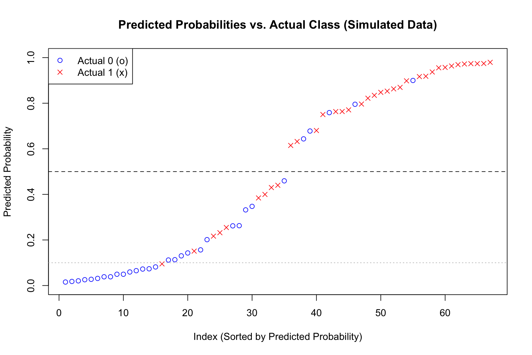
Plotting the Predictive Probabilities with True Labels
Code
## --- 5. Plot sorted predicted probabilities ---## Create a data frame for plottingplot_data_sim <-data.frame(Prob = pred_probs_sim,Actual =as.factor(test_data_sim$y),TrueProb = test_data_sim$p # Include true probs for comparison)## Sort by predicted probabilityplot_data_sim <- plot_data_sim[order(plot_data_sim$Prob), ]plot_data_sim$Rank <-1:nrow(plot_data_sim)## Create the plotplot( plot_data_sim$Rank, plot_data_sim$Prob,pch =ifelse(plot_data_sim$Actual ==0, 1, 4),col =ifelse(plot_data_sim$Actual ==0, "blue", "red"),xlab ="Index (Sorted by Predicted Probability)",ylab ="Predicted Probability",main ="Predicted Probabilities vs. Actual Class (Simulated Data)",ylim =c(0, 1))abline(h =0.5, lty =2, col ="black")abline(h =0.1, lty =3, col ="grey")## Add the true probability curve (sorted by predicted prob)## This shows how well the fitted model's predictions align with the true probs#lines(plot_data_sim$Rank, plot_data_sim$TrueProb[order(plot_data_sim$Prob)], col = "darkgreen", lwd = 2)## Add a legendlegend("topleft",legend =c("Actual 0 (o)", "Actual 1 (x)"),pch =c(1, 4),lty =c(NA, NA),lwd =c(NA, NA),col =c("blue", "red"))
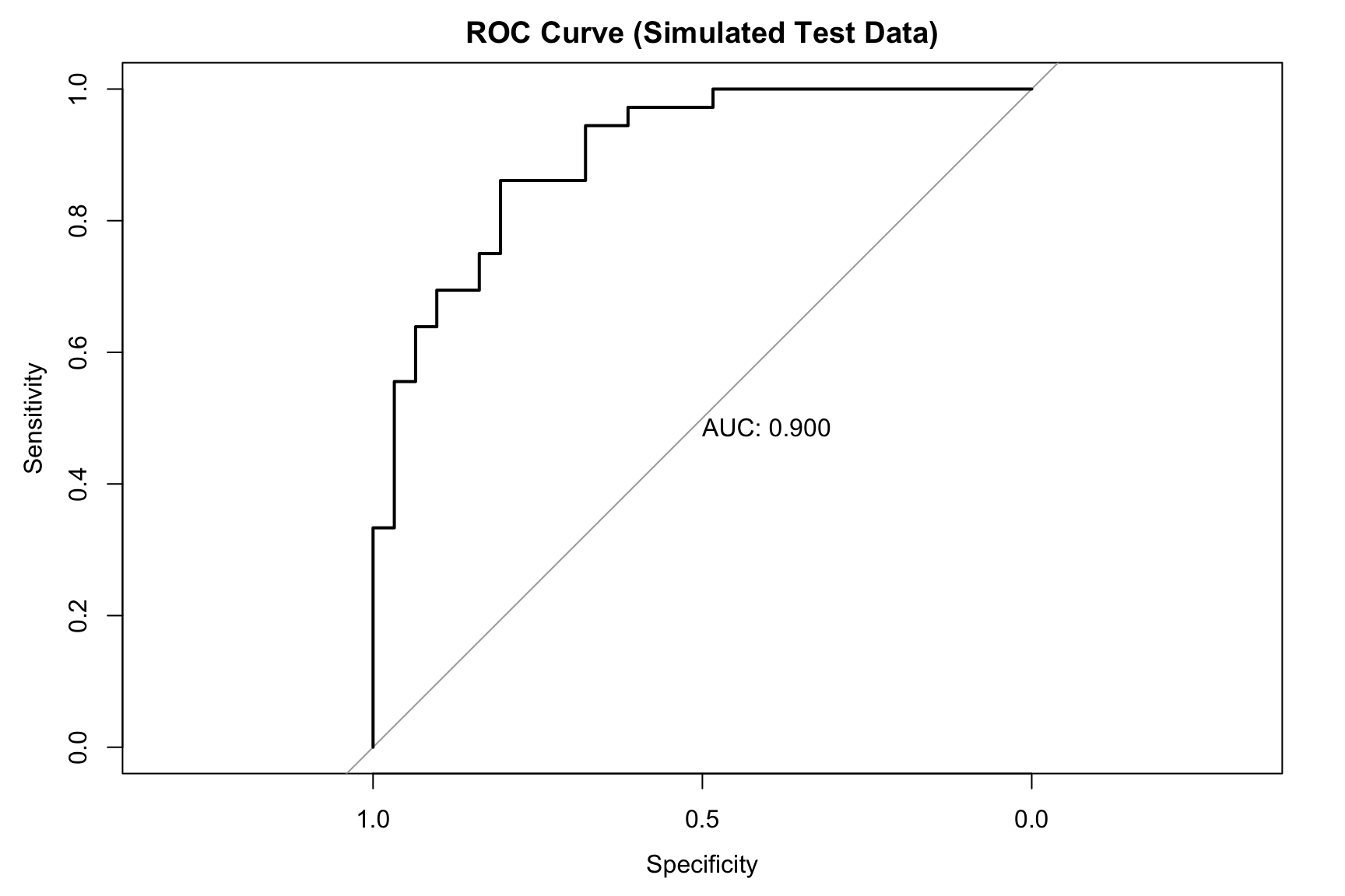
## 4b. Area Under the Curve (AUC)roc_curve_sim <-roc(test_data_sim$y, pred_probs_sim, quiet =TRUE)## Plot the ROC curveplot(roc_curve_sim, main ="ROC Curve (Simulated Test Data)", print.auc =TRUE)
Code
auc_value_sim <-auc(roc_curve_sim)cat(paste("Area Under the Curve (AUC):", round(auc_value_sim, 4), "\n\n"))
Area Under the Curve (AUC): 0.8996
PR curve and Area Under PR Curve (AUPR)
Code
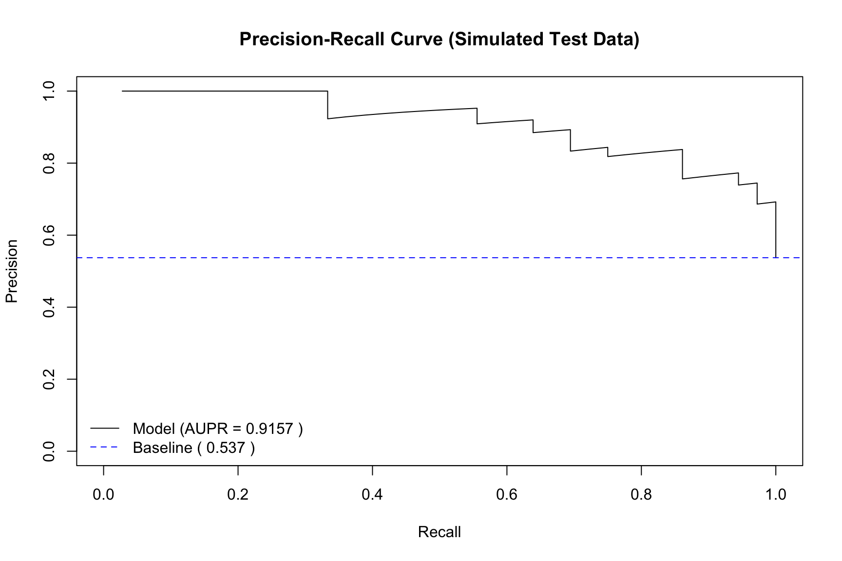
## Load the ROCR library## install.packages("ROCR") # Uncomment to install if neededlibrary(ROCR)## --- 1. Create a 'prediction' object ---## 'prediction' takes all predictions and all true labelspred_obj <-prediction(pred_probs_sim, test_data_sim$y)## --- 2. Create a 'performance' object for PR ---## "prec" is for precision, "rec" is for recallperf_pr <-performance(pred_obj, measure ="prec", x.measure ="rec")## --- 3. Calculate Area Under the PR Curve (AUPR) ---perf_auc <-performance(pred_obj, measure ="aucpr") # "aucpr" = Area Under PR Curveaupr_value <- perf_auc@y.values[[1]]cat(paste("Area Under PR Curve (AUPR):", round(aupr_value, 4), "\n"))
Area Under PR Curve (AUPR): 0.9157
Code
## --- 4. Plot the performance object ---plot(perf_pr, main ="Precision-Recall Curve (Simulated Test Data)", xlim =c(0, 1), ylim =c(0, 1),col ="black")## --- 5. Calculate and add the 'no-skill' baseline ---baseline_precision_sim <-sum(test_data_sim$y ==1) /length(test_data_sim$y)abline(h = baseline_precision_sim, col ="blue", lty =2)## --- 6. Add a legend with AUPR ---legend("bottomleft", legend =c(paste("Model (AUPR =", round(aupr_value, 4), ")"), # <-- MODIFIED LINEpaste("Baseline (", round(baseline_precision_sim, 3), ")") ), col =c("black", "blue"), lty =c(1, 2), bty ="n") # bty="n" removes the box
6.8.3 Application to the CHD Dataset
Code
## Load the pROC library for AUC calculation## install.packages("pROC") # Uncomment to install if neededlibrary(pROC)## --- 1. Split the data ---set.seed(123) # for reproducibilityn <-nrow(CHD.data)train_size <-floor(2/3* n)train_indices <-sample(1:n, size = train_size)train_data <- CHD.data[train_indices, ]test_data <- CHD.data[-train_indices, ]## --- 2. Refit the model on the training data ---fit_train <-glm( chd ~ smk + cat + sbp + age + chl + ecg + hpt,data = train_data,family =binomial(link ="logit"))## --- 3. Make predictions on the test data ---pred_probs <-predict(fit_train, newdata = test_data, type ="response")
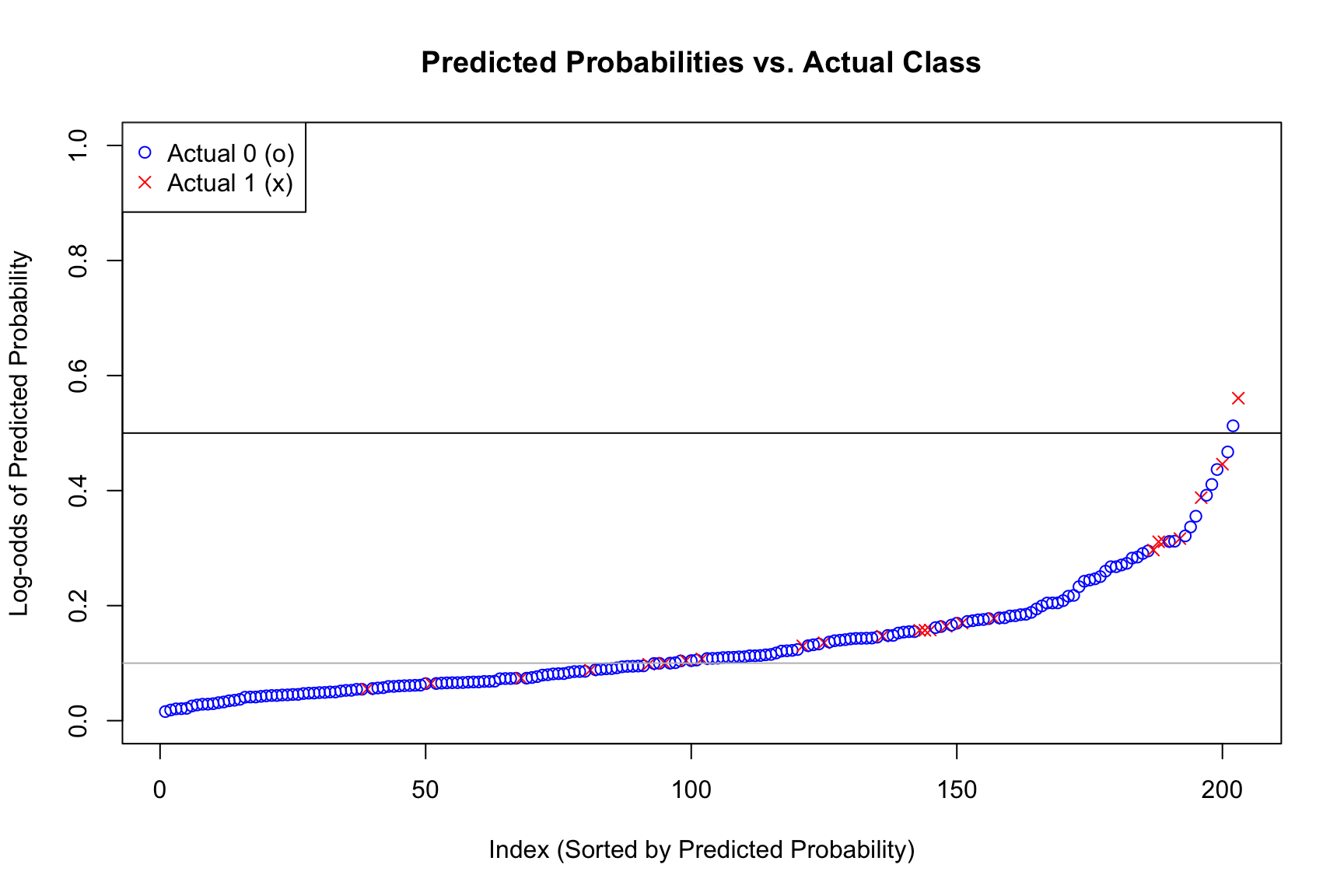
Plot Predictive Probabilities
Code
## --- 5. Plot sorted predicted probabilities ---## Create a data frame for plottingplot_data <-data.frame(Prob = pred_probs,Actual =as.factor(test_data$chd))## Sort by predicted probabilityplot_data <- plot_data[order(plot_data$Prob), ]plot_data$Rank <-1:nrow(plot_data)## Create the plot## We use 'pch' (plot character) to set different symbols## 'pch = 1' is 'o' (default)## 'pch = 4' is 'x'plot( plot_data$Rank, plot_data$Prob,pch =ifelse(plot_data$Actual ==0, 1, 4),col =ifelse(plot_data$Actual ==0, "blue", "red"),xlab ="Index (Sorted by Predicted Probability)",ylab ="Log-odds of Predicted Probability",main ="Predicted Probabilities vs. Actual Class",ylim =c(0,1))abline(h=0.5)abline(h=0.1, col="grey")## Add a legendlegend("topleft",legend =c("Actual 0 (o)", "Actual 1 (x)"),pch =c(1, 4),col =c("blue", "red"))
ROC curve and Area Under the ROC (AUC)
Code
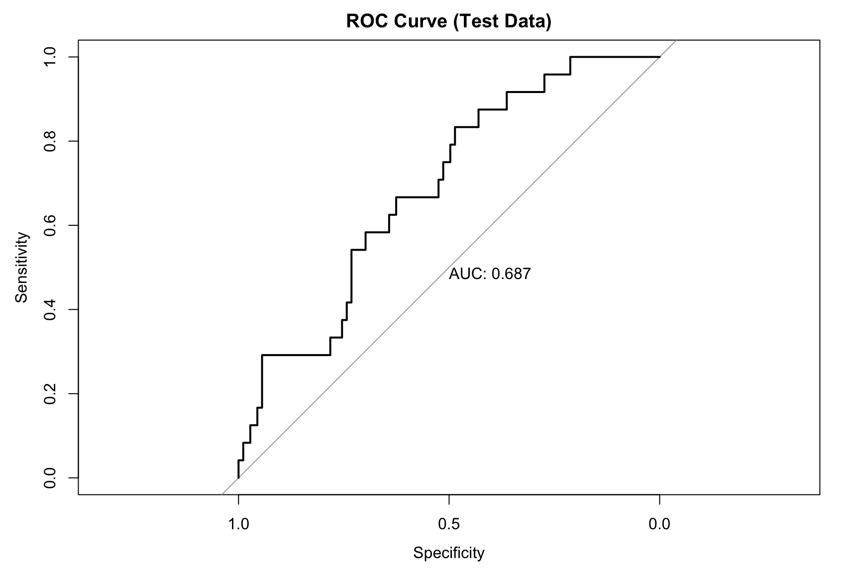
## 4b. Area Under the Curve (AUC)roc_curve <-roc(test_data$chd, pred_probs, quiet =TRUE)## Plot the ROC curveplot(roc_curve, main ="ROC Curve (Test Data)", print.auc =TRUE)
Code
auc_value <-auc(roc_curve)cat(paste("Area Under the Curve (AUC):", round(auc_value, 4), "\n\n"))
Area Under the Curve (AUC): 0.6872
PR curve and Area Under PR Curve (AUPR)
Code
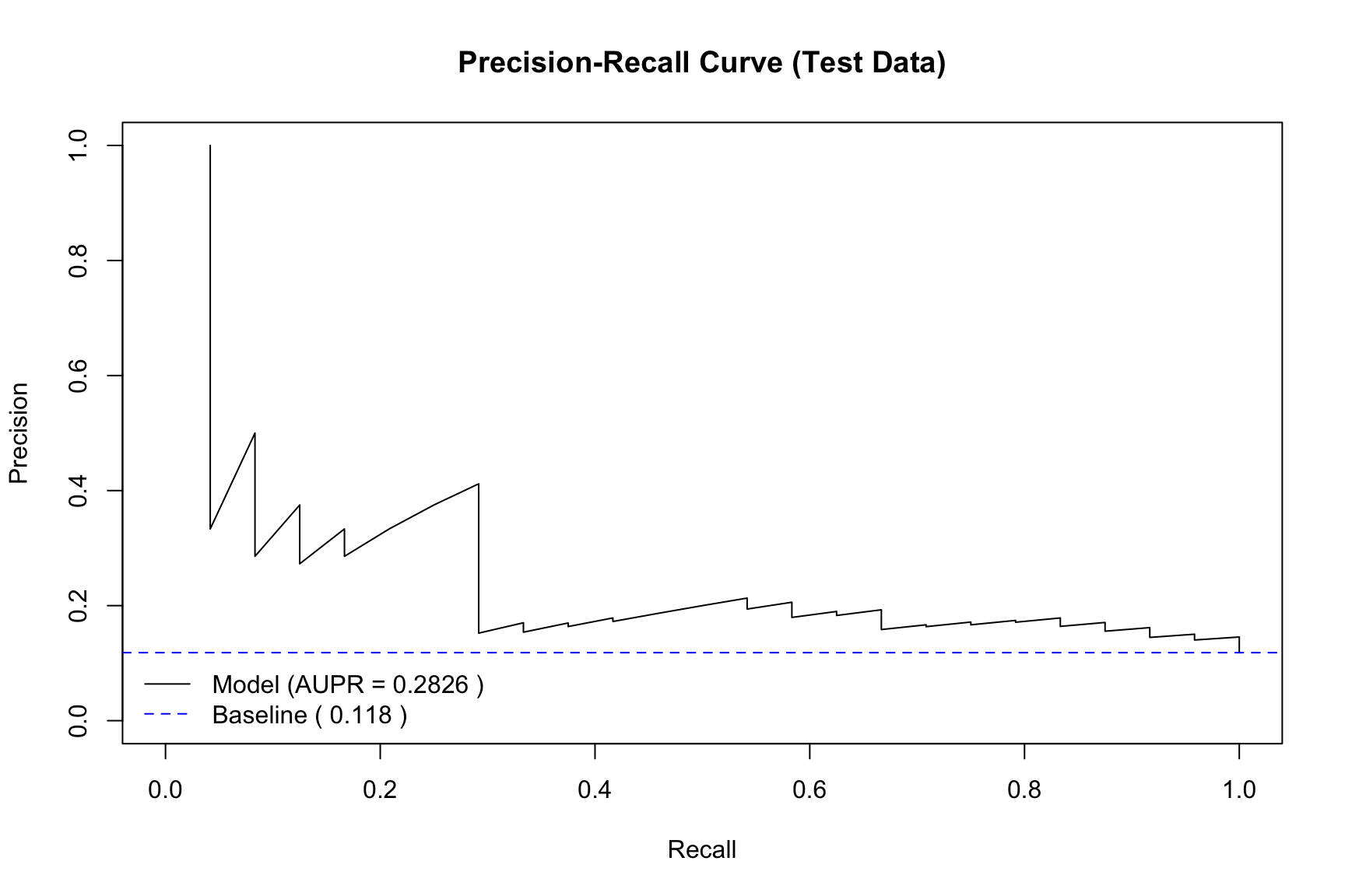
## Load the ROCR library## install.packages("ROCR") # Uncomment to install if neededlibrary(ROCR)## --- 1. Create a 'prediction' object ---## 'prediction' takes all predictions and all true labels## We use 'pred_probs' and 'test_data$chd' from the CHD data splitpred_obj <-prediction(pred_probs, test_data$chd)## --- 2. Create a 'performance' object for PR ---## "prec" is for precision, "rec" is for recallperf_pr <-performance(pred_obj, measure ="prec", x.measure ="rec")## --- 3. Calculate Area Under the PR Curve (AUPR) ---perf_auc <-performance(pred_obj, measure ="aucpr") # "aucpr" = Area Under PR Curveaupr_value <- perf_auc@y.values[[1]]cat(paste("Area Under PR Curve (AUPR):", round(aupr_value, 4), "\n"))
Area Under PR Curve (AUPR): 0.2826
Code
## --- 4. Plot the performance object ---plot(perf_pr, main ="Precision-Recall Curve (Test Data)", xlim =c(0, 1), ylim =c(0, 1),col ="black")## --- 5. Calculate and add the 'no-skill' baseline ---baseline_precision <-sum(test_data$chd ==1) /length(test_data$chd)abline(h = baseline_precision, col ="blue", lty =2)## --- 6. Add a legend with AUPR ---legend("bottomleft", legend =c(paste("Model (AUPR =", round(aupr_value, 4), ")"), # <-- MODIFIED LINEpaste("Baseline (", round(baseline_precision, 3), ")") ), col =c("black", "blue"), lty =c(1, 2), bty ="n") # bty="n" removes the box